Advanced Oscilloscope Tips: Trigger/Decode/Automated Measurements - Let the Waveforms Speak for Themselves

Introduction

When I first got my oscilloscope, I thought as long as I could see the waveform, everything was fine. Until one day I was debugging a strange SPI communication issue - the waveform “looked normal” but the device just wouldn’t work. Later, a senior engineer told me: “You’re using the oscilloscope as a multimeter!”

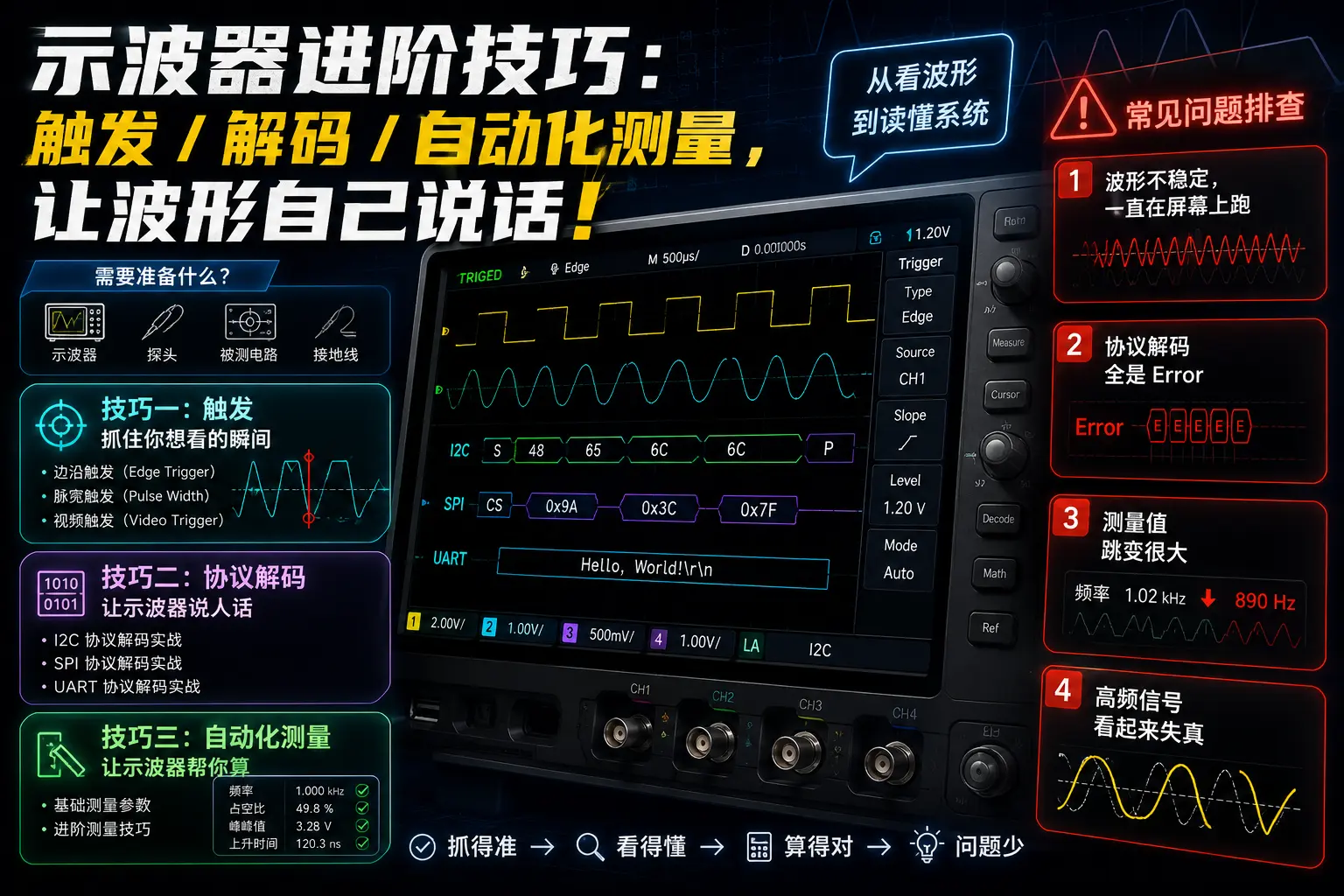
Today we’re going to talk about advanced oscilloscope techniques. Not teaching you how to turn it on and see waveforms, but how to make the oscilloscope help you “read” signals. After mastering these techniques, you’ll find that the same equipment can reveal completely different amounts of information.

What Do You Need to Prepare?

Item	Model/Specification	Price
Digital Oscilloscope	Any model with trigger/decode support	¥800-5000
Passive Probe	100MHz, 10:1	¥50-150
Logic Analyzer	Saleae Logic 8 or compatible	¥200-400
Test Signal Source	Signal generator or development board	¥100-300
Jumper Wires/Test Clips	Several	¥20
Total		¥1170-5870

💡 Tip: If you don’t have a professional signal source, using Arduino/ESP32 to generate test signals is perfectly adequate.

Tip 1: Triggering - Capturing the Moment You Want to See

Why is Triggering Important?

Imagine you’re taking photos on a highway, trying to capture a red car. If you just press the shutter randomly, you might capture any vehicle. But if you set it to “only press shutter when you see a red car,” your success rate is much higher.

That’s exactly how oscilloscope triggering works. The default auto-run mode (Auto) is like pressing the shutter randomly - the waveform runs all over the screen, and you can’t see the details clearly at all.

Edge Trigger - Most Basic but Most Practical

Trigger Type: Edge
Trigger Source: CH1
Trigger Edge: Rising
Trigger Level: 1.5V

Practical Scenario: Capturing the start bit of UART serial data.

UART is high level when idle, and the start bit is a falling edge. After setting falling edge trigger, every time data is sent, the oscilloscope will stably display the complete frame.

⚠️ Pitfall Warning: Set the trigger level between 30%-70% of the signal amplitude. Set it too high and it may never trigger; set it too low and it will trigger falsely.

Pulse Width Trigger - Catching Abnormal Pulses

Trigger Type: Pulse Width
Trigger Condition: Less Than
Time Threshold: 100ns

Practical Scenario: Glitch interference on power supply.

Normal power supply signals are stable, but occasionally there are narrow pulse interferences. Using pulse width trigger set to “pulses less than 100ns,” you can catch these occasional anomalies.

I once debugged a system that kept restarting, and using this method I caught a 50ns power supply glitch - it turned out to be coupling interference from the switching instant of a certain MOS transistor.

Video Trigger - Analyzing Video Signals

Trigger Type: Video
Standard: NTSC/PAL
Line/Field: Field (Field Sync)

Practical Scenario: Debugging camera output or old-style CRT displays.

Video signals have strict synchronization timing. Using video trigger can directly lock onto field sync or line sync, making it convenient to measure video timing parameters.

Tip 2: Protocol Decoding - Making the Oscilloscope Speak Human Language

Why Do We Need Protocol Decoding?

When looking at SPI waveforms, what you see is:

CH1: ████▁▁████▁▁▁███▁████▁▁▁
CH2: ▁███▁▁▁████▁████▁▁███▁▁▁

What can you tell from this? Nothing at all!

After enabling SPI decoding, the oscilloscope will tell you:

SPI: 0x5A 0x3C 0xFF 0x01

Now that’s human-readable!

I2C Protocol Decoding in Practice

Wiring:

• CH1 → SCL (clock line)

• CH2 → SDA (data line)

Decoding Settings:

Protocol Type: I2C
Clock Source: CH1
Data Source: CH2
Rate: 100kHz (standard mode) or 400kHz (fast mode)
Display Format: Hex (hexadecimal) or ASCII

Practical Case: Debugging MPU6050 Accelerometer

Decoding Results:
START | ADDR+W | ACK | REG(0x75) | ACK | STOP
START | ADDR+R | ACK | DATA(0x68) | NACK | STOP

From this decoding you can see:

1. I2C start signal successfully sent, bus enters communication state

2. Slave address 0x68 correctly addressed, device responded with ACK

3. WHO_AM_I register (0x75) returned 0x68, consistent with datasheet, indicating normal communication

• Whether probe ground is good

• Whether trigger level is appropriate

• Whether I2C bus has pull-up resistors (4.7kΩ-10kΩ)

SPI Protocol Decoding in Practice

Wiring:

• CH1 → SCK (clock)

• CH2 → MOSI (master output)

• CH3 → MISO (master input)

• CH4 → CS (chip select, optional)

Decoding Settings:

Protocol Type: SPI
Clock Source: CH1
MOSI Source: CH2
MISO Source: CH3
Chip Select Source: CH4 (if available)
Clock Polarity: CPOL=0 (idle low)
Clock Phase: CPHA=1 (sample on second edge)

⚠️ How to Determine CPOL/CPHA? Check the chip datasheet! If set incorrectly, all decoded data will be wrong.

UART Protocol Decoding in Practice

Wiring:

• CH1 → TX (transmit end)

Decoding Settings:

Protocol Type: UART/RS232
Signal Source: CH1
Baud Rate: 9600/115200 (according to actual settings)
Data Bits: 8
Parity: None
Stop Bits: 1

Practical Tip: UART decoding can directly display ASCII characters, very convenient for debugging serial logs.

Decoding Display:
 System initialized
 Temperature: 25.6°C
 Battery low: 3.2V

Tip 3: Automated Measurements - Let the Oscilloscope Do the Calculations for You

Basic Measurement Parameters

Modern digital oscilloscopes all come with measurement functions, no need to manually count divisions:

Measurement Item    Typical Value    Description
─────────────────────────────────────
Frequency (Freq)    1.000 kHz        Reciprocal of signal period
Period              1.000 ms         Complete waveform time
Rise Time           25.3 ns          10%-90% amplitude time
Fall Time           28.1 ns          90%-10% amplitude time
Pulse Width         500.2 μs         High level duration
Duty Cycle          50.1 %           High level ratio
Maximum (Max)       3.28 V           Highest point of waveform
Minimum (Min)       -0.02 V          Lowest point of waveform
Peak-to-Peak (Vpp)  3.30 V           Max - Min
Average (Mean)      1.65 V           DC component
RMS (Vrms)          1.17 V           AC RMS value

Advanced Measurement Techniques

1. Enable Measurement Statistics

After enabling statistics, the oscilloscope will record multiple measurements of:

• Average (Mean)

• Standard Deviation (Std Dev)

• Maximum (Max)

• Minimum (Min)

Practical Application: Measuring power supply ripple stability. The smaller the standard deviation of ripple voltage, the more stable the power supply.

2. Using Cursors for Precise Measurements

Cursor Type: Time Cursor (ΔT)
Cursor A: 1.000 ms
Cursor B: 1.250 ms
Difference ΔT: 250.0 μs

Practical Scenario: Measuring the time interval between two events, such as the setup time from CS going low to the first SCK edge.

3. Mathematical Operation Functions

Operation Type: CH1 - CH2
Purpose: Differential signal analysis

Operation Type: FFT (Fast Fourier Transform)
Purpose: Frequency domain analysis, finding noise frequency components

Practical Case: Power supply noise analysis. Looking in the time domain shows a messy waveform, but looking at FFT, you find a spike at 50kHz - it turns out the switching power supply’s switching frequency is coupling in.

Common Problem Troubleshooting

Problem 1: Waveform is Unstable, Keeps Running Across the Screen

Cause: Improper trigger settings or no trigger

Solution:

1. Confirm trigger source selection is correct (corresponds to the channel where the signal is)

2. Adjust trigger level to between 30%-70% of signal amplitude

3. Change trigger mode from Auto to Normal to avoid free scanning when there’s no trigger

4. Check if probe ground is reliable; ground leads that are too long will introduce noise causing false triggering

Cause: Decoding parameters don’t match actual signal

Solution:

1. Verify if baud rate/clock frequency matches decoding settings

2. Check if polarity/phase parameters like CPOL/CPHA match the chip datasheet

3. Confirm probe ground is good, signal edges are clean without glitches

4. Try increasing sampling rate to ensure protocol edges are fully sampled

Cause: Signal itself is unstable or measurement setup issues

Solution:

1. Enable multiple measurement statistics, use average and standard deviation to evaluate stability

2. Check if probe connections are secure; loose connections will cause contact resistance jumps

3. Confirm if the signal itself is stable - verify oscilloscope is working normally with an external signal source

4. Appropriately increase sampling depth and sampling rate to improve measurement accuracy

Cause: Oscilloscope bandwidth insufficient or probe settings wrong

Solution:

1. Confirm oscilloscope bandwidth ≥ 5 times the signal frequency (rule of thumb)

2. Check if probe attenuation ratio settings match oscilloscope channel settings (1:1 or 10:1)

3. Perform probe compensation calibration to ensure square wave edges have no overshoot or rounding

4. Use the shortest possible ground spring instead of long ground leads to reduce high-frequency loop inductance

The oscilloscope is the hardware engineer’s eyes, but many people only use 10% of its capabilities. The three advanced techniques discussed today:

1. Make good use of trigger functions - edge, pulse width, video trigger to precisely locate target events

2. Enable protocol decoding - let the oscilloscope directly “speak” I2C/SPI/UART data content

3. Utilize automated measurements and FFT - hand over tedious manual calculations to the oscilloscope, doubling efficiency

After mastering these, you’ll find debugging efficiency greatly improved. Problems that used to take half an hour to analyze can now be located in 5 minutes.

Finally, a suggestion: when buying an oscilloscope, don’t just look at bandwidth and sampling rate. The support for trigger functions and protocol decoding often determines the actual user experience more.

Hope this blog post is helpful to you!

---

Related Resources:

• Oscilloscope Probe Compensation Calibration Tutorial

• I2C Protocol Explained in Detail

• SPI Communication Debugging Guide

• Hardware I2C Debugging Tips: Logic Analyzer Packet Capture in Practice