2026年8月9日 OpenCV

Complete Guide to OpenCV Python Image Processing: Color, Channels, Histograms, Morphology, Masks

1. Introduction

OpenCV (Open Source Computer Vision Library) is one of the most widely used open-source libraries in computer vision, and Python is its most popular binding. In everyday image processing work, we frequently need to perform various fundamental operations on images: color space conversion, channel splitting and merging, masking and bitwise operations, flipping and resizing, gamma correction, histogram analysis, morphological operations, and data type conversion.

Many tutorials cover only one of these operations in isolation, lacking a comprehensive reference that ties them all together. This guide consolidates more than 10 of the most commonly used OpenCV Python image processing operations into a single article, with runnable code examples, parameter explanations, and notes for each. Whether you’re an OpenCV beginner or a developer looking to systematically review image processing knowledge, this guide serves as a handy reference.

The OpenCV version used in this guide is 4.1.1 and above, running in Jupyter Notebook, with all example images displayed via Matplotlib.

2. Environment Setup

2.1 Installing Dependencies

pip install opencv-python numpy matplotlib

2.2 Loading Libraries and Sample Images

All examples below assume the following imports:

import cv2            # OpenCV
import numpy as np    # NumPy for numerical computing
import matplotlib.pyplot as plt  # Image display

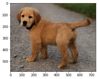
Load and display a sample image:

img = cv2.imread("dog.png")
img = cv2.cvtColor(img, cv2.COLOR_BGR2RGB)
plt.imshow(img)
plt.title("Original")
plt.axis("off")
plt.show()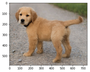

Original

Important Note: OpenCV’s cv2.imread() reads images in BGR color space by default, while Matplotlib’s plt.imshow() expects RGB data. If you display an OpenCV-loaded image directly in Jupyter Notebook, the colors will be wrong (red appears blue, blue appears red). The fix is to convert using cv2.cvtColor(img, cv2.COLOR_BGR2RGB).

3. Color Space Conversion with cv.cvtColor

3.1 Function Syntax

dst = cv2.cvtColor(src, code[, dst[, dstCn]])

src: Input image matrix (image data read via cv2.imread())
code: Color space conversion flag, specifying the source and target color spaces
dst (optional): Output image, same width and height as src
dstCn (optional): Number of channels in the output image; 0 means same as src

3.2 BGR to RGB

This is the most commonly needed conversion for Jupyter Notebook users. Skipping it causes incorrect colors.

img_bgr2rgb = cv2.cvtColor(img, cv2.COLOR_BGR2RGB)
plt.imshow(img_bgr2rgb)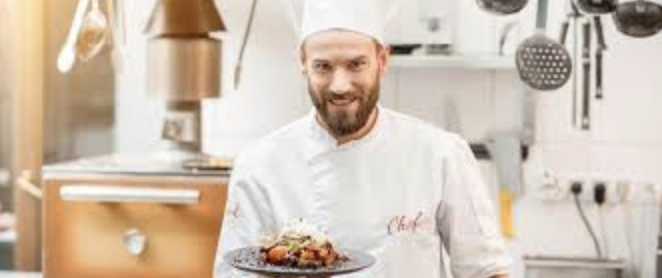

BGR to RGB

3.3 BGR to HSV

HSV (Hue, Saturation, Value) color space is very useful for color detection and color segmentation tasks.

img_bgr2hsv = cv2.cvtColor(img, cv2.COLOR_BGR2HSV)
plt.imshow(img_bgr2hsv)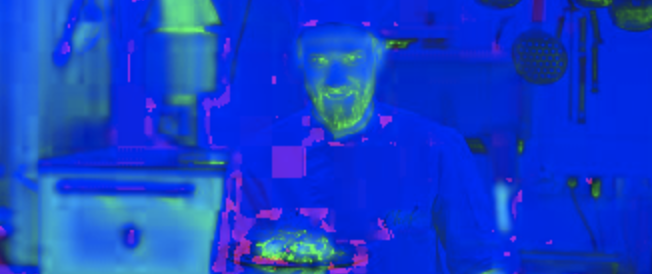

BGR to HSV

3.4 BGR to Grayscale

img_rgb2gray = cv2.cvtColor(img, cv2.COLOR_RGB2GRAY)
plt.imshow(img_rgb2gray, cmap="gray")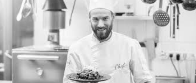

Grayscale

Note: When displaying grayscale images, always include the cmap="gray" parameter. Otherwise, Matplotlib will use its default pseudocolor mapping (colormap), causing the grayscale image to appear yellowish-green or other incorrect colors. This is one of the most common beginner mistakes.

3.5 Why Do We Need Different Color Spaces?

Different color spaces suit different tasks:

BGR/RGB: Suitable for standard image display and storage; the native format for most image files. BGR is OpenCV’s legacy default, while RGB is the standard for web and most display devices.
Grayscale (GRAY): Only one channel, lower computational cost, suitable for edge detection, thresholding, and other tasks that don’t need color information. Many classic algorithms (like Canny edge detection) require grayscale input.
HSV: Separates color information (hue, saturation) from brightness (value), making it ideal for color-based object detection and segmentation. For example, detecting red objects only requires setting a red range in the H channel, unaffected by lighting changes.
HLS: Similar to HSV, but the L (lightness) channel is more thoroughly separated from color, yielding better results in certain image enhancement scenarios.
YCrCb: Commonly used in video encoding and face detection, where Y represents luminance and Cr/Cb represent chrominance. OpenCV’s Haar face detector operates in YCrCb space.

3.6 Quick Reference for Common Color Space Conversion Flags

Flag	Meaning
`cv2.COLOR_BGR2RGB`	BGR → RGB
`cv2.COLOR_BGR2GRAY`	BGR → Grayscale
`cv2.COLOR_BGR2HSV`	BGR → HSV
`cv2.COLOR_BGR2HLS`	BGR → HLS
`cv2.COLOR_BGR2YCrCb`	BGR → YCrCb
`cv2.COLOR_HSV2BGR`	HSV → BGR

4. Channel Operations

A color image is represented as a 3D NumPy array with shape (height, width, channels). The last dimension represents channels — for RGB images, channel 0 is R (red), channel 1 is G (green), and channel 2 is B (blue).

4.1 Direct Channel Manipulation with NumPy

img = cv2.imread('dog.png').astype(np.float32) / 255
img = cv2.cvtColor(img, cv2.COLOR_BGR2RGB)

# Swap the red and blue channels
img[:, :, [0, 2]] = img[:, :, [2, 0]]
plt.imshow(img)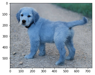

Channel Swap

After swapping, the image takes on BGR-mode colors with noticeable color distortion. Performing the same operation again swaps them back.

4.2 Scaling Individual Channels

# Reduce the red channel by 10%
img[:, :, 0] = (img[:, :, 0] * 0.9).clip(0, 1)
# Increase the green channel by 10%
img[:, :, 1] = (img[:, :, 1] * 1.1).clip(0, 1)

plt.imshow(img)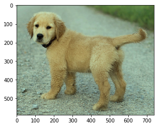

Green Channel Enhanced

The resulting image appears greenish because the green channel was boosted and the red channel was reduced.

4.3 Using cv2.split and cv2.merge

# Split channels
b, g, r = cv2.split(img)

# Merge channels
img_merged = cv2.merge([r, g, b])

cv2.split returns multiple single-channel arrays, while cv2.merge combines multiple single-channel arrays into a multi-channel image. Both approaches and NumPy indexing have their use cases — NumPy is more flexible (allows direct algebraic operations), while cv2.split/merge offers clearer semantics.

5. Image Masking and Binary Operations

Masks are a crucial concept in image processing. Binary images contain only black and white pixel values (0 and 255). Both OpenCV and NumPy support all common binary operators: NOT, AND, OR, and XOR.

5.1 Creating Masks

# Create a 500x500 black image with a white circle
circle_image = np.zeros((500, 500), np.uint8)
cv2.circle(circle_image, (250, 250), 100, 255, -1)

# Create a 500x500 black image with a white rectangle
rect_image = np.zeros((500, 500), np.uint8)
cv2.rectangle(rect_image, (100, 100), (400, 250), 255, -1)

5.2 Binary Operations

# AND operation
circle_and_rect_image = circle_image & rect_image
# Equivalent to cv2.bitwise_and(circle_image, rect_image)

# OR operation
circle_or_rect_image = circle_image | rect_image
# Equivalent to cv2.bitwise_or(circle_image, rect_image)

# NOT operation
not_image = cv2.bitwise_not(circle_image)
# Equivalent to ~circle_image

# XOR operation
xor_image = cv2.bitwise_xor(circle_image, rect_image)
# Equivalent to circle_image ^ rect_image

5.3 Displaying Results

plt.figure(figsize=(10, 10))
plt.subplot(221)
plt.axis('off')
plt.title('circle')
plt.imshow(circle_image, cmap='gray')
plt.subplot(222)
plt.axis('off')
plt.title('rectangle')
plt.imshow(rect_image, cmap='gray')
plt.subplot(223)
plt.axis('off')
plt.title('circle & rectangle')
plt.imshow(circle_and_rect_image, cmap='gray')
plt.subplot(224)
plt.axis('off')
plt.title('circle | rectangle')
plt.imshow(circle_or_rect_image, cmap='gray')
plt.tight_layout()
plt.show()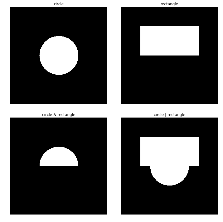

Mask Operation Results

Using np.uint8 arrays with values 0 and 255 to represent binary images is very convenient. These operations are commonly used in practice to extract Regions of Interest (ROI). For example: using bitwise_and with a mask on the original image preserves only the content in the white (masked) area.

5.4 Practical Application of Masks: Extracting Regions of Interest

The most common use of masks is extracting specific areas from an image. Given an irregularly shaped foreground mask, we can use it to keep only the foreground:

# Load the original image (color)
img = cv2.imread('dog.png')
img_rgb = cv2.cvtColor(img, cv2.COLOR_BGR2RGB)

# Create a mask the same size as the image (assuming we have a mask)
# White areas (255) are kept, black areas (0) are removed
mask = np.zeros(img.shape[:2], dtype=np.uint8)
cv2.circle(mask, (200, 200), 150, 255, -1)  # Circular mask

# Use bitwise_and to extract the masked region
# Note: For color images, the mask must be passed via the mask parameter
masked_img = cv2.bitwise_and(img_rgb, img_rgb, mask=mask)

plt.imshow(masked_img)
plt.title('Mask Extraction Result')
plt.show()

Mask operations are common in the following scenarios:

Image segmentation: Extracting segmented target regions with masks
Background removal: Creating a foreground mask and performing AND with the original image
Regional statistics: Computing mean, histograms, and other statistics within masked areas
Image compositing: Blending two images according to a mask

6. Image Flipping with cv.flip

6.1 Function Syntax

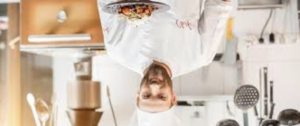
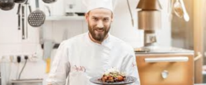
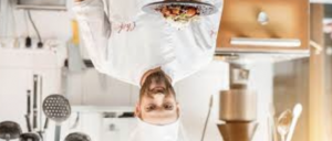
dst = cv2.flip(src, flipCode[, dst])

src: Input image
flipCode: Flip flag
- 0: Flip around the X-axis (vertical flip / top-bottom flip)
- Positive (e.g., 1): Flip around the Y-axis (horizontal flip / left-right flip)
- Negative (e.g., -1): Flip around both axes (equivalent to 180° clockwise rotation)

6.2 Code Example

img = cv2.imread("cook.jpeg")
img = cv2.cvtColor(img, cv2.COLOR_BGR2RGB)

# Vertical flip
img_flip_vertical = cv2.flip(img, 0)

# Horizontal flip
img_flip_horizontal = cv2.flip(img, 1)

# Flip both axes (180° rotation)
img_flip_both = cv2.flip(img, -1)

Flip Mode	flipCode	Effect
Vertical flip	0	Upside down
Horizontal flip	1	Left-right mirror
Both axes flip	-1	Upside down + mirrored (= 180° rotation)

Vertical Flip

Horizontal Flip

Both Axes Flip

7. Image Resizing with cv2.resize

7.1 Function Syntax

dst = cv2.resize(src, dsize[, dst[, fx[, fy[, interpolation]]]])

src: Input image
dsize: Output image size (width, height); if (0, 0), computed from fx and fy
fx: Horizontal scale factor
fy: Vertical scale factor
interpolation: Interpolation method

7.2 Resizing to Specific Dimensions

img = cv2.imread("cook.jpeg")
height, width, channel = img.shape
print('Original size:', img.shape)  # (147, 342, 3)

# Scale down by half
resized_img = cv2.resize(img, (width // 2, height // 2))
print('Resized down:', resized_img.shape)  # (73, 171, 3)

# Scale up by 2x
resized_img = cv2.resize(img, (width * 2, height * 2))
print('Resized up:', resized_img.shape)  # (294, 684, 3)

7.3 Scaling by Factor

w_mult, h_mult = 0.25, 0.5
resized_img = cv2.resize(img, (0, 0), fx=w_mult, fy=h_mult)
print('Scaled size:', resized_img.shape)  # (74, 86, 3)

7.4 Interpolation Methods

Method	Description	Best For
`cv2.INTER_NEAREST`	Nearest neighbor	Fastest, lowest quality, visible pixelation
`cv2.INTER_LINEAR`	Bilinear interpolation (default)	Recommended for upscaling
`cv2.INTER_CUBIC`	Bicubic interpolation	Better quality for upscaling, slower
`cv2.INTER_AREA`	Area-based interpolation	Recommended for downscaling, avoids aliasing

# Using nearest-neighbor interpolation
resized_img = cv2.resize(img, (0, 0), fx=0.25, fy=0.5, interpolation=cv2.INTER_NEAREST)

Best Practice: Use cv2.INTER_AREA for downscaling and cv2.INTER_CUBIC or cv2.INTER_LINEAR for upscaling. INTER_NEAREST is fastest but lowest quality — typically only used when speed is critical and quality doesn’t matter.

8. Gamma Correction

8.1 Principle

Gamma correction is a non-linear operation used to adjust pixel intensity. Its formula is:

$$V_{out} = V_{in}^{\gamma}$$

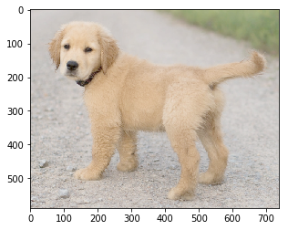
When $\gamma < 1$: image becomes brighter (shadow details are lifted)
When $\gamma > 1$: image becomes darker (highlights are compressed)
When $\gamma = 1$: output equals input, no change

Gamma correction is important in display calibration, image enhancement, HDR processing, and more.

8.2 Code Implementation

First normalize pixel values to the 0–1 range, then use np.power for the exponentiation.

# Load image, convert to float32 and normalize to 0-1
img = cv2.imread('dog.png').astype(np.float32) / 255
img = cv2.cvtColor(img, cv2.COLOR_BGR2RGB)

# gamma = 0.5, image brightens
gamma = 0.5
corrected_bright = np.power(img, gamma)
plt.imshow(corrected_bright)
plt.title("gamma=0.5 (brighter)")
plt.show()

# gamma = 1.5, image darkens
gamma = 1.5
corrected_dark = np.power(img, gamma)
plt.imshow(corrected_dark)
plt.title("gamma=1.5 (darker)")
plt.show()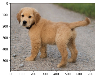

Original

gamma=0.5 brighter

gamma=1.5 darker

Note: np.power requires input values in the 0–1 range, so normalization is mandatory. Using raw uint8 values (0–255) for exponentiation will cause overflow.

8.3 Practical Applications of Gamma Correction

Gamma correction is more than just “making images brighter or darker.” Its core idea is to model the human eye’s non-linear perception of brightness. The human eye is more sensitive to changes in dark areas than bright ones, and displays themselves have gamma characteristics (typically around 2.2).

Common applications include:

Image preprocessing: Using gamma correction before OCR, edge detection, etc., to ensure proper brightness
Exposure compensation: Using $\gamma < 1$ to brighten underexposed photos, $\gamma > 1$ to darken overexposed ones
Display calibration: Correcting the gamma response curve of display devices
Medical imaging: Enhancing subtle contrast differences in X-rays and other medical images
Data augmentation: In deep learning, gamma correction is often used as a data augmentation technique — randomly selecting $\gamma$ values to increase model robustness to lighting variations

9. Image Mean and Standard Deviation

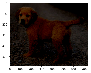
The mean of an image reflects its overall brightness, while the standard deviation reflects the dispersion of pixel values (i.e., contrast). Standardizing an image matrix (subtracting the mean, dividing by the standard deviation) is a common preprocessing step for many computer vision algorithms.

9.1 Computing with NumPy

img = cv2.imread('dog.png').astype(np.float32) / 255
img = cv2.cvtColor(img, cv2.COLOR_BGR2RGB)

# Compute mean
mean_val = img.mean()
print(f"Mean: {mean_val}")

# Subtract mean to get zero-mean matrix
mean_img = img.copy()
mean_img -= mean_img.mean()

# Compute standard deviation
std_val = std_img.std()
print(f"Std: {std_val}")

# Divide by std to get unit-variance matrix
std_img = mean_img.copy()
std_img /= std_img.std()

9.2 Using cv2.mean and cv2.meanStdDev

# cv2.mean returns the mean of each channel
mean_per_channel = cv2.mean(img)
print(f"Per-channel mean: {mean_per_channel}")

# cv2.meanStdDev returns both mean and std in one call
mean, stddev = cv2.meanStdDev(img)
print(f"Mean: {mean.flatten()}")
print(f"Std: {stddev.flatten()}")

9.3 NumPy Equivalents

# Equivalent to cv2.mean
np_mean = np.mean(img, axis=(0, 1))

# Equivalent to cv2.meanStdDev
np_std = np.std(img, axis=(0, 1))

Application: Zero-mean unit-variance standardization is a common deep learning image preprocessing step. It normalizes the data distribution across different images, aiding model convergence. After mean subtraction, the image appears grayish — this is normal, as it removes overall brightness and preserves only relative differences.

Zero-mean image

Unit-variance image

10. Histograms

A histogram is a statistical chart showing the distribution of pixel values in an image. It can quickly reveal whether an image is overexposed (pixels concentrated on the right) or underexposed (pixels concentrated on the left).

10.1 Computing Histograms with np.histogram

img = cv2.imread('dog.png')
img = cv2.cvtColor(img, cv2.COLOR_BGR2RGB)

# Compute histogram
hist, bins = np.histogram(img, 256, [0, 255])

# Display histogram
plt.fill(hist)
plt.xlabel('pixel value')
plt.show()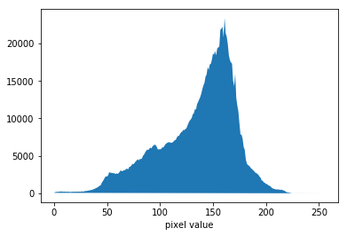

Histogram

np.histogram parameters:

a: Input array
bins: Number of bins
range: Value range (min, max)
Returns: (hist, bin_edges) — histogram array and bin edges

10.2 Using cv2.calcHist

OpenCV provides a dedicated histogram computation function cv2.calcHist:

# Grayscale histogram
gray = cv2.cvtColor(img, cv2.COLOR_BGR2GRAY)
hist = cv2.calcHist([gray], [0], None, [256], [0, 256])

# Plot histogram
plt.plot(hist)
plt.xlabel('pixel value')
plt.ylabel('count')
plt.show()

10.3 Grayscale Histogram Equalization

The goal of histogram equalization is to normalize image brightness and enhance contrast.

# Read in grayscale mode
img_gray = cv2.imread('dog.png', 0)

# Equalize
img_gray_eq = cv2.equalizeHist(img_gray)

# Display result
plt.figure(figsize=(12, 4))
plt.subplot(121)
plt.imshow(img_gray, cmap='gray')
plt.title('Original')
plt.subplot(122)
plt.imshow(img_gray_eq, cmap='gray')
plt.title('Equalized')
plt.show()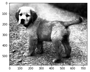

Equalization Comparison

The equalized histogram shows a more uniform distribution:

hist, bins = np.histogram(img_gray_eq, 256, [0, 255])
plt.fill_between(range(256), hist, 0)
plt.xlabel('pixel value')
plt.show()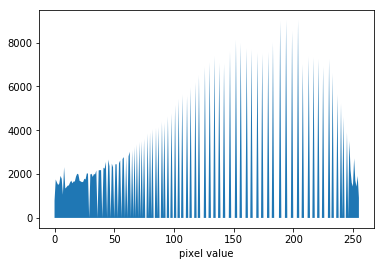

Equalized Histogram

10.4 Color Image Histogram Equalization

cv2.equalizeHist only accepts single-channel images. For color images, equalize each of the R, G, B channels separately:

img_color = cv2.imread('dog.png')
img_color = cv2.cvtColor(img_color, cv2.COLOR_BGR2RGB)

# Equalize each of the R, G, B channels
img_color[..., 0] = cv2.equalizeHist(img_color[..., 0])  # R channel
img_color[..., 1] = cv2.equalizeHist(img_color[..., 1])  # G channel
img_color[..., 2] = cv2.equalizeHist(img_color[..., 2])  # B channel

plt.imshow(img_color)
plt.title('Color Equalization')
plt.show()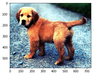

Color Equalization

Advanced Tip: For color images, it’s better to equalize in HSV space — equalizing only the V (value) channel enhances contrast without distorting colors, then convert back to RGB.

10.5 Histogram Equalization in HSV Space

Compared to equalizing all three RGB channels separately, equalizing only the V channel in HSV space produces better results because it doesn’t change the image’s colors (H and S channels remain unchanged), only adjusting the brightness distribution:

img = cv2.imread('dog.png')
img_hsv = cv2.cvtColor(img, cv2.COLOR_BGR2HSV)

# Equalize only the V (value) channel
img_hsv[:, :, 2] = cv2.equalizeHist(img_hsv[:, :, 2])

# Convert back to BGR then to RGB for display
img_result = cv2.cvtColor(img_hsv, cv2.COLOR_HSV2BGR)
img_result = cv2.cvtColor(img_result, cv2.COLOR_BGR2RGB)

plt.imshow(img_result)
plt.title('HSV Space Equalization')
plt.show()

10.6 CLAHE: Adaptive Histogram Equalization

Global histogram equalization can sometimes over-enhance — contrast in certain regions gets amplified too much. OpenCV provides CLAHE (Contrast Limited Adaptive Histogram Equalization), which divides the image into tiles and equalizes each separately, then uses bilinear interpolation to eliminate tile boundaries while limiting contrast amplification to avoid excessive noise enhancement:

img_gray = cv2.imread('dog.png', 0)

# Create CLAHE object
# clipLimit controls contrast limiting (default 40.0) — higher = more contrast enhancement
# tileGridSize defines tile size (default 8x8)
clahe = cv2.createCLAHE(clipLimit=2.0, tileGridSize=(8, 8))

# Apply CLAHE
img_clahe = clahe.apply(img_gray)

plt.imshow(img_clahe, cmap='gray')
plt.title('CLAHE Equalization')
plt.show()

CLAHE almost always outperforms global histogram equalization in practice, especially in scenes with both very bright and very dark areas. It’s the go-to method for medical image enhancement and low-light image enhancement.

11. Morphological Operations

Mathematical morphology can be understood as a filtering operation, hence it’s also called morphological filtering. The filters (kernels) used are called structuring elements in morphology, typically shaped as rectangles, ellipses, crosses, etc.

11.1 Constructing Binary Images

import cv2
import numpy as np
import matplotlib.pyplot as plt

img = cv2.imread('dog.png', 0)

# Use Otsu's method to automatically determine the threshold for binarization
_, binary = cv2.threshold(img, -1, 1, cv2.THRESH_BINARY | cv2.THRESH_OTSU)

11.2 Erosion and Dilation

# Erode 10 times with a 3x3 rectangular structuring element
eroded = cv2.morphologyEx(binary, cv2.MORPH_ERODE, (3, 3), iterations=10)

# Dilate 10 times with a 3x3 rectangular structuring element
dilated = cv2.morphologyEx(binary, cv2.MORPH_DILATE, (3, 3), iterations=10)

11.3 Opening and Closing

# Opening with a 5x5 elliptical structuring element, 5 iterations (erode then dilate)
opened = cv2.morphologyEx(binary, cv2.MORPH_OPEN,
                          cv2.getStructuringElement(cv2.MORPH_ELLIPSE, (5, 5)),
                          iterations=5)

# Closing with a 5x5 elliptical structuring element, 5 iterations (dilate then erode)
closed = cv2.morphologyEx(binary, cv2.MORPH_CLOSE,
                          cv2.getStructuringElement(cv2.MORPH_ELLIPSE, (5, 5)),
                          iterations=5)

11.4 Morphological Gradient, Top-Hat, and Black-Hat

# Morphological gradient: highlights blob edges, preserves object contours
grad = cv2.morphologyEx(binary, cv2.MORPH_GRADIENT,
                        cv2.getStructuringElement(cv2.MORPH_ELLIPSE, (5, 5)))

# Top-hat: highlights regions brighter than surroundings
tophat = cv2.morphologyEx(binary, cv2.MORPH_TOPHAT,
                          cv2.getStructuringElement(cv2.MORPH_ELLIPSE, (5, 5)))

# Black-hat: highlights regions darker than surroundings
blackhat = cv2.morphologyEx(binary, cv2.MORPH_BLACKHAT,
                            cv2.getStructuringElement(cv2.MORPH_ELLIPSE, (5, 5)))

11.5 Morphological Operations Quick Reference

Operation	Flag	Formula	Purpose
Erosion	`MORPH_ERODE`	—	Remove small white dots, shrink objects
Dilation	`MORPH_DILATE`	—	Remove small black dots, expand objects
Opening	`MORPH_OPEN`	Erode then dilate	Remove small white dots, separate objects, smooth edges
Closing	`MORPH_CLOSE`	Dilate then erode	Fill small black holes, connect adjacent objects
Morphological gradient	`MORPH_GRADIENT`	Dilate − Erode	Highlight edge contours
Top-hat	`MORPH_TOPHAT`	Original − Opening	Highlight bright details
Black-hat	`MORPH_BLACKHAT`	Closing − Original	Highlight dark details

Morphological Operation Results

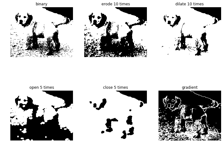
11.6 Structuring Element Creation

# Rectangular structuring element
kernel_rect = cv2.getStructuringElement(cv2.MORPH_RECT, (5, 5))

# Elliptical structuring element
kernel_ellipse = cv2.getStructuringElement(cv2.MORPH_ELLIPSE, (5, 5))

# Cross-shaped structuring element
kernel_cross = cv2.getStructuringElement(cv2.MORPH_CROSS, (5, 5))

11.7 Practical Applications of Morphological Operations

Morphological operations are widely used in real projects. Here are some typical scenarios:

1. Noise Removal (Opening) In document scanning or OCR preprocessing, binarized images often have small noise spots. Opening (erode then dilate) effectively removes these white dots without changing the shape and size of the main text regions.

2. Connecting Broken Regions (Closing) In license plate detection, characters may be broken due to poor image quality. Closing (dilate then erode) can reconnect broken strokes.

3. Extracting Object Contours (Morphological Gradient) The morphological gradient equals dilation minus erosion, highlighting object edges. This is useful when traditional edge detection doesn’t work well for extracting object boundaries.

4. Uneven Illumination Correction (Top-Hat Transform) When image background illumination is uneven, the top-hat transform can extract small bright targets (e.g., bright spots on a dark background), commonly used in microscopy image analysis.

5. Extracting Dark Details (Black-Hat Transform) The black-hat transform extracts small dark targets, useful for detecting dark blemishes or defects on bright backgrounds.

Choosing structuring element size and iteration count is key to morphological operations. Larger elements and more iterations produce stronger effects, but over-processing destroys image structure. It’s generally recommended to start small (3×3) and increase gradually based on results.

12. Data Type Conversion

Image data is typically stored as uint8 (0–255) or float32 (0.0–1.0). Different operations have different data type requirements:

cv2.imread() returns uint8 by default
Many mathematical operations (gamma correction, standardization, etc.) require float32
cv2.imshow() expects uint8 (0–255) or float32 (0.0–1.0)
Bitwise operations (bitwise_and, etc.) require uint8

12.1 uint8 → float32

img = cv2.imread('dog.png')
print('Original type:', img.dtype)  # uint8

# Convert to float32 and normalize to 0-1
img_float = img.astype(np.float32) / 255
print('Converted type:', img_float.dtype)  # float32

12.2 float32 → uint8

# Multiply by 255 to restore 0-255 range, then convert to uint8
img_uint8 = (img_float * 255).astype(np.uint8)
print('Restored type:', img_uint8.dtype)  # uint8

12.3 Using np.clip to Prevent Overflow

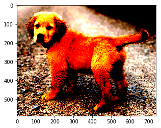
# Multiply each element by 2, clip to 0-1 range
img_clip = np.clip(img_float * 2, 0, 1)
plt.imshow(img_clip)
plt.title('Overexposed (value×2)')
plt.show()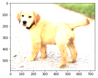

Overexposed Effect

Key Warning: When performing arithmetic on uint8, values exceeding 255 don’t get clipped — they wrap around (e.g., 200 + 100 = 44). Before algebraic operations, convert to float32, then convert back to uint8 afterward, or use safe methods like np.clip / cv2.add.

12.4 Other Data Types

Besides uint8 and float32, OpenCV supports these image data types:

Data Type	Value Range	Description
`uint8`	0 – 255	Most common image format, 8-bit unsigned integer
`uint16`	0 – 65535	Used in medical imaging, depth maps, RAW images
`int32`	-2^31 – 2^31-1	Occasionally used for signed intermediate results like gradients
`float32`	0.0 – 1.0	Common in mathematical operations and deep learning
`float64`	Same, higher precision	Used in scientific computing, larger memory footprint

12.5 Safe Conversion with cv2.convertScaleAbs

OpenCV provides cv2.convertScaleAbs to perform scaling, offset, and type conversion in one step:

# Convert float32 image (0-1) back to uint8 (0-255)
img_uint8 = cv2.convertScaleAbs(img_float, alpha=255, beta=0)

# Equivalent to:
# img_uint8 = np.clip(img_float * 255, 0, 255).astype(np.uint8)

This function handles clipping and type conversion internally, making it safer than manual operations. alpha is the scale factor, beta is the offset.

13. Comprehensive Example

Below is a comprehensive example chaining multiple operations into a typical image processing pipeline:

import cv2
import numpy as np
import matplotlib.pyplot as plt

# Step 1: Load image and convert data type
img = cv2.imread('dog.png').astype(np.float32) / 255
img = cv2.cvtColor(img, cv2.COLOR_BGR2RGB)

# Step 2: Gamma correction (brighten)
gamma_corrected = np.power(img, 0.7)

# Step 3: Adjust channel color balance
gamma_corrected[:, :, 0] = (gamma_corrected[:, :, 0] * 0.95).clip(0, 1)  # R slightly down
gamma_corrected[:, :, 1] = (gamma_corrected[:, :, 1] * 1.05).clip(0, 1)  # G slightly up

# Step 4: Convert back to uint8 for further processing
img_uint8 = (gamma_corrected * 255).astype(np.uint8)

# Step 5: Convert to grayscale and apply histogram equalization
gray = cv2.cvtColor(img_uint8, cv2.COLOR_RGB2GRAY)
gray_eq = cv2.equalizeHist(gray)

# Step 6: Binarize + morphological operations
_, binary = cv2.threshold(gray_eq, 0, 255, cv2.THRESH_BINARY + cv2.THRESH_OTSU)
kernel = cv2.getStructuringElement(cv2.MORPH_ELLIPSE, (3, 3))
opened = cv2.morphologyEx(binary, cv2.MORPH_OPEN, kernel, iterations=2)

# Step 7: Extract foreground using mask
foreground = cv2.bitwise_and(img_uint8, img_uint8, mask=opened)

# Step 8: Display results
plt.figure(figsize=(16, 12))
plt.subplot(231); plt.imshow(img); plt.title('1. Original'); plt.axis('off')
plt.subplot(232); plt.imshow(gamma_corrected); plt.title('2. Gamma + Channel Adjust'); plt.axis('off')
plt.subplot(233); plt.imshow(gray_eq, cmap='gray'); plt.title('3. Equalized Grayscale'); plt.axis('off')
plt.subplot(234); plt.imshow(binary, cmap='gray'); plt.title('4. Binarized (Otsu)'); plt.axis('off')
plt.subplot(235); plt.imshow(opened, cmap='gray'); plt.title('5. Morphological Opening'); plt.axis('off')
plt.subplot(236); plt.imshow(foreground); plt.title('6. Mask-Extracted Foreground'); plt.axis('off')
plt.tight_layout()
plt.show()

This example demonstrates a complete workflow: data type conversion → color space transformation → channel operations → gamma correction → histogram equalization → binarization → morphological operations → mask extraction. Each step builds on the previous result, representing a common image processing pipeline in real projects.

13.1 Common Image Processing Pipeline Patterns

In real projects, different tasks typically follow different processing patterns. Here are several common pipeline combinations:

Document Scanning / OCR Preprocessing Pipeline: Color space to grayscale → Gaussian blur denoising → Adaptive threshold binarization → Morphological opening for noise removal → Perspective transform correction

Color Detection Pipeline: BGR → HSV color space conversion → Create mask by setting color range in H channel → Morphological operations to smooth mask → bitwise_and to extract target region

Image Enhancement Pipeline: Gamma correction for brightness adjustment → CLAHE for local contrast enhancement → Channel balance adjustment → Sharpening filter

Object Detection Preprocessing Pipeline: Resize image to fixed dimensions → Convert data type to float32 → Zero-mean unit-variance standardization → Feed into detection model

14. Summary

This guide covers 13 core OpenCV Python image processing operations:

#	Operation	Core Function
1	Color space conversion	`cv2.cvtColor()`
2	Channel operations	`cv2.split()`, `cv2.merge()`, NumPy indexing
3	Masking & binary operations	`cv2.bitwise_and/or/not/xor()`
4	Image flipping	`cv2.flip()`
5	Image resizing	`cv2.resize()`
6	Gamma correction	`np.power()`
7	Mean & standard deviation	`cv2.mean()`, `cv2.meanStdDev()`, NumPy
8	Histogram computation	`np.histogram()`, `cv2.calcHist()`
9	Histogram equalization	`cv2.equalizeHist()`
10	Morphological operations	`cv2.morphologyEx()`
11	Data type conversion	`.astype()`, `np.clip()`
12	Binarization	`cv2.threshold()`
13	Comprehensive pipeline	Combining the above operations

Key Takeaways

BGR vs RGB: OpenCV reads as BGR, Matplotlib needs RGB — don’t forget cv2.cvtColor
Grayscale display: Matplotlib needs cmap="gray" for grayscale images
Data type safety: Convert to float32 before arithmetic, convert back after, use np.clip to prevent overflow
Interpolation choice: Use INTER_AREA for downscaling, INTER_CUBIC or INTER_LINEAR for upscaling
Equalization tips: For color images, equalize the V channel in HSV space for more natural results
Morphology applications: Opening for noise removal, closing for hole filling, gradient for edge extraction — structuring element size and shape affect results

I hope this comprehensive guide becomes your go-to reference for daily image processing work. If you have any questions, feel free to discuss in the comments.

Recommended Learning Path

If you’re new to OpenCV, I recommend learning and practicing in this order:

Phase 1 (Fundamentals): Environment setup → Image loading & display → Color space conversion → Image flipping & resizing
Phase 2 (Channels & Masks): Channel operations → Data type conversion → Binary operations & masking
Phase 3 (Image Analysis): Histogram computation → Histogram equalization / CLAHE → Mean & standard deviation
Phase 4 (Advanced): Gamma correction → Morphological operations → Comprehensive pipelines

It’s recommended to learn and practice in Jupyter Notebook at each phase, testing different parameters with various images. Image processing is a highly practical discipline — just reading code isn’t enough. Adjusting parameters yourself and observing the effects is the only way to truly understand each operation’s principles and use cases.