OpenCV Python 轮廓与矩阵实战：NumPy 矩阵操作 + findContours 详解

引言

在 OpenCV Python 中，图像的本质就是 NumPy 多维数组（也称为矩阵或张量）。无论是简单的像素赋值、通道分离，还是复杂的轮廓检测与形状分析，所有操作的底层都是对矩阵的运算。因此，在深入学习轮廓检测之前，掌握 NumPy 矩阵的基本操作是必不可少的。本文将从矩阵基础出发，逐步过渡到 cv2.findContours 的完整实战，帮助你建立从像素到轮廓的完整认知链路。

第一部分：NumPy 图像矩阵操作

本示例使用的 OpenCV 版本是：4.1.1，运行环境为 Jupyter Notebook 6.0.0。

1. 加载依赖库

import cv2
import numpy as np
import matplotlib.pyplot as plt

2. 矩阵的核心概念

图像矩阵有两个关键特征——形状（shape）和数据类型（dtype）：

• shape：矩阵的维度信息。例如一个 480×640 的 3 通道图像，其 shape 为 (480, 640, 3)，分别表示高度、宽度和通道数。
• dtype：矩阵中每个元素的数据类型。np.uint8 表示每个元素占 8 位无符号整数，取值范围为 0～255。

3. 使用 np.full 创建矩阵

# 创建一个 480x640 的 3 通道矩阵，用 255 填充——得到一张纯白色图像
image = np.full((480, 640, 3), 255, np.uint8)

plt.figure(figsize=(9, 9))
plt.imshow(image)

注意：figsize 以英寸为单位定义图像窗口大小（1 英寸 = 2.54 厘米），设置较大的值可以让图像显示得更清晰。

4. 指定通道值创建彩色图像

# 第三通道设为 255，在 BGR 模式下代表红色
image = np.full((480, 640, 3), (0, 0, 255), np.uint8)

# matplotlib 使用 RGB 色彩空间，需要先做 BGR→RGB 转换
image = cv2.cvtColor(image, cv2.COLOR_BGR2RGB)

plt.figure(figsize=(9, 9))
plt.imshow(image)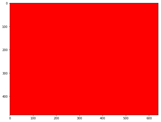

5. 使用 fill 填充矩阵

# 用 0 填充整个矩阵——得到一张纯黑色图像
image.fill(0)

plt.figure(figsize=(9, 9))
plt.imshow(image)

6. 指定元素赋值——单点操作

# 将三个指定坐标的像素设为白色
image[240, 160] = image[240, 320] = image[240, 480] = (255, 255, 255)

plt.figure(figsize=(9, 9))
plt.imshow(image)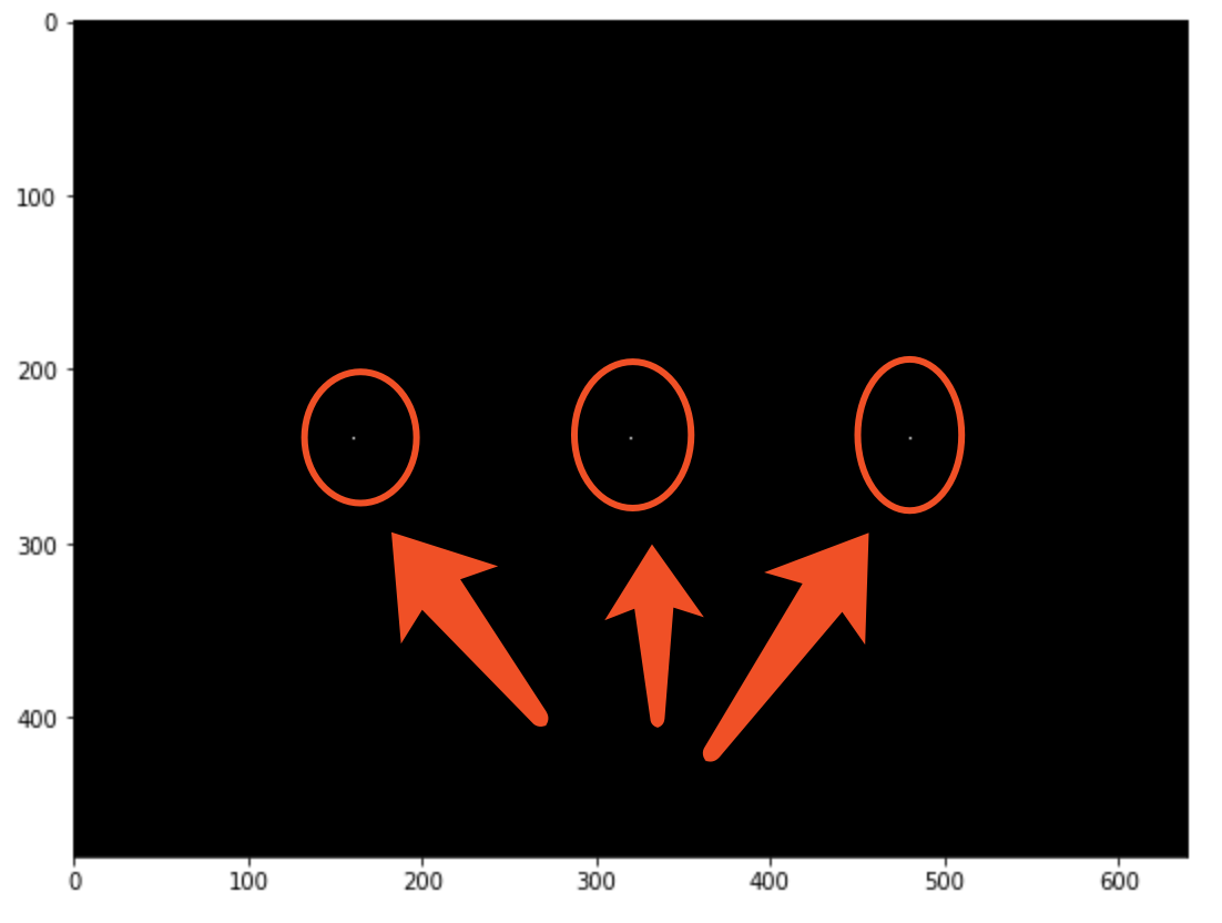

仔细查看图片，可以看到 3 个白色像素点，恰好位于 [240, 160]、[240, 320]、[240, 480] 这三个坐标位置。

7. 指定元素赋值——整通道操作

# 将第一个通道全部设为 255（在 RGB 模式下显示为红色）
image[:, :, 0] = 255

plt.figure(figsize=(9, 9))
plt.imshow(image)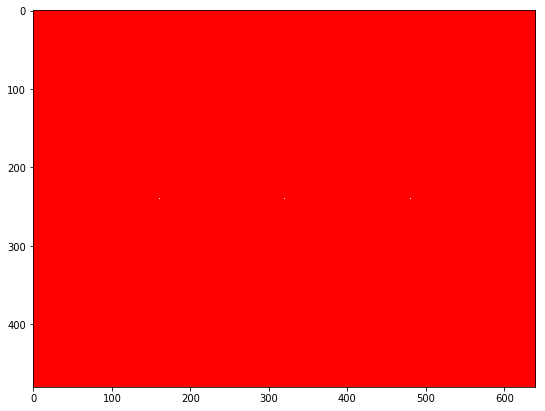

注意：仔细观察仍然可以看到之前设置的 3 个白色像素点，因为它们的三个通道都已经是 255。

8. 指定元素赋值——垂直线操作

# 将图像中间垂直线上所有像素设为白色
image[:, 320, :] = 255

plt.figure(figsize=(9, 9))
plt.imshow(image)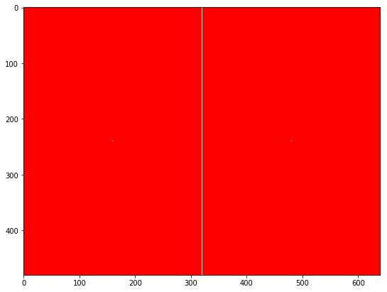

9. 指定元素赋值——区域 + 通道操作

# 在区域 [100:600, 100:200] 内，将通道索引 2 的值设为 255
# 通道索引 2 在 RGB 中是蓝色通道，红色 + 蓝色 = 紫红色
image[100:600, 100:200, 2] = 255

plt.figure(figsize=(9, 9))
plt.imshow(image)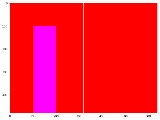

矩阵操作小结

操作	语法	说明
访问元素	image[240, 160]	返回该像素的三通道值数组
访问单通道	image[240, 160, 1]	返回该像素第二通道的值
全行/列选择	image[:, 160]	y 为 160 的所有像素
区域选择	image[120:140, 160]	x 为 120～140，y 为 160 的区域
整通道赋值	image[:, :, 0] = 255	第一个通道全部设为 255

NumPy 支持高维数组与矩阵运算，也提供了大量数学函数库。在使用 PyTorch 等深度学习框架时，NumPy 数组还可以非常方便地转换成张量交给 GPU 处理。

第二部分：轮廓检测 findContours

什么是轮廓？

轮廓可以简单地解释为连接具有相同颜色或强度的所有连续点（沿边界）的曲线。轮廓是用于形状分析以及对象检测和识别的有用工具。

为了获得更高的准确性，使用二进制图像效果会更佳。因此，在找到轮廓之前，请先使用阈值处理或 Canny 边缘检测。自从 OpenCV 3.2，findContours() 不再修改原图片，因此不需要事先复制一份。

在 OpenCV 中，找到轮廓就像从黑色背景中找到白色物体——要找到的对象应该是白色，背景应该是黑色。

基本用法

import numpy as np
import cv2 as cv

im = cv.imread('test.jpg')
imgray = cv.cvtColor(im, cv.COLOR_BGR2GRAY)
ret, thresh = cv.threshold(imgray, 127, 255, 0)
contours, hierarchy = cv.findContours(thresh, cv.RETR_TREE, cv.CHAIN_APPROX_SIMPLE)

程序先读入 test.jpg，转成灰度图，以 127 作为阈值进行二值化处理，再执行轮廓查找。

cv.findContours() 有三个参数：

1. 源图像：输入的二值图像。
2. 轮廓检索模式：
   • RETR_EXTERNAL — 仅检索最外部轮廓
   • RETR_LIST — 检索所有轮廓而不建立任何层次关系
   • RETR_CCOMP — 检索所有轮廓并将它们组织成两级层次结构。顶层是组件的外部边界，第二层是孔的边界
   • RETR_TREE — 检索所有轮廓并重建嵌套轮廓的完整层次结构
   • RETR_FLOODFILL — 多级图像的连通分量
3. 轮廓逼近方法（详见下文）。

返回值 contours 是一个 Python 列表，每个元素是对象边界点的 (x, y) 坐标的 NumPy 数组。hierarchy 描述轮廓之间的嵌套关系。

绘制轮廓

使用 cv.drawContours() 函数绘制轮廓：

# 绘制所有轮廓
cv.drawContours(img, contours, -1, (0, 255, 0), 3)

# 绘制第 4 个轮廓
cv.drawContours(img, contours, 3, (0, 255, 0), 3)

# 更常用的方式：先取出轮廓再绘制
cnt = contours[4]
cv.drawContours(img, [cnt], 0, (0, 255, 0), 3)

轮廓逼近方法

这是 cv.findContours 的第三个参数，决定轮廓是否存储所有边界点：

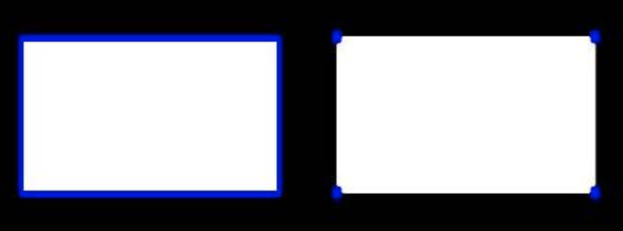
• cv.CHAIN_APPROX_NONE：存储所有边界点。
• cv.CHAIN_APPROX_SIMPLE：删除冗余点并压缩轮廓，节省内存。例如一条直线只需保留两个端点。

下面的矩形图像直观地演示了差异：CHAIN_APPROX_NONE 得到 734 个点，而 CHAIN_APPROX_SIMPLE 只得到 4 个点——内存节省效果非常显著！

不同阈值的实战对比

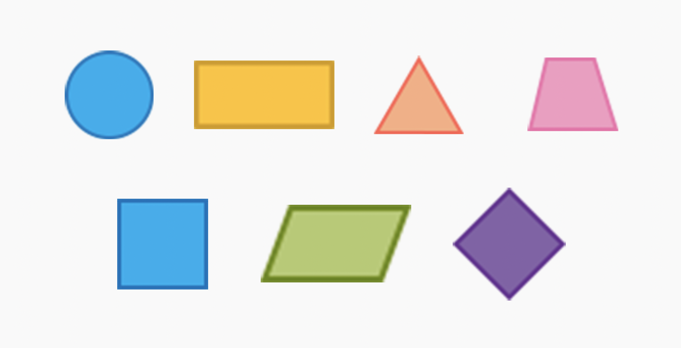
我们以一幅包含多种形状的图像为例，对比不同阈值参数下的轮廓检测效果。

原图：

参数：阈值=127，轮廓检索模式=RETR_TREE，轮廓逼近方法=CHAIN_APPROX_SIMPLE

原图	灰度处理后	阈值处理后	画出轮廓

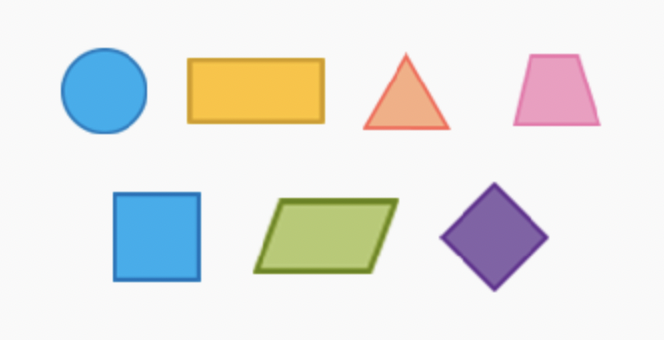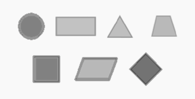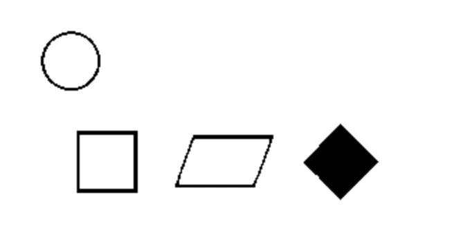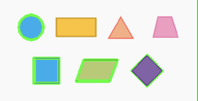从处理结果可以看到，因为阈值过低，导致偏暖色的形状被过滤，无法正确获取所有轮廓。

参数：阈值=200，轮廓检索模式=RETR_TREE，轮廓逼近方法=CHAIN_APPROX_SIMPLE

原图	灰度处理后	阈值处理后	画出轮廓

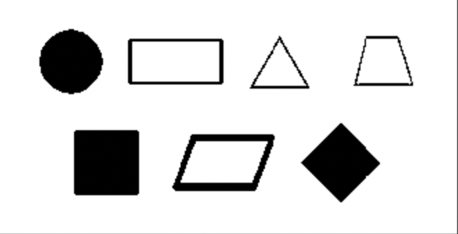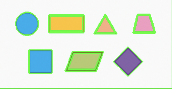虽然这次把所有轮廓都画出来了，但也发现了另一个问题：整幅图的边缘和某些形状的内圈也被画上了轮廓。

至于这些轮廓之间的顺序关系，我们将在后续文章中详细讨论。

第三部分：矩阵 + 轮廓综合实战

理解了矩阵操作和轮廓检测之后，我们可以将两者结合起来：用 NumPy 创建图像矩阵并绘制形状，然后用 findContours 检测这些形状的轮廓。

import numpy as np
import cv2 as cv
import matplotlib.pyplot as plt

# 1. 用 NumPy 创建一张黑色背景图像
image = np.full((480, 640, 3), 0, np.uint8)

# 2. 在矩阵上绘制白色形状
cv.rectangle(image, (50, 50), (200, 200), (255, 255, 255), -1)    # 白色矩形
cv.circle(image, (400, 240), 100, (255, 255, 255), -1)             # 白色圆形
cv.line(image, (250, 400), (550, 400), (255, 255, 255), 3)         # 白色线段

# 3. 转灰度 + 阈值处理
gray = cv.cvtColor(image, cv.COLOR_BGR2GRAY)
ret, thresh = cv.threshold(gray, 127, 255, 0)

# 4. 查找并绘制轮廓
contours, hierarchy = cv.findContours(thresh, cv.RETR_TREE, cv.CHAIN_APPROX_SIMPLE)
cv.drawContours(image, contours, -1, (0, 255, 0), 2)

# 5. 显示结果
plt.figure(figsize=(9, 9))
plt.imshow(cv2.cvtColor(image, cv.COLOR_BGR2RGB))
plt.title(f'Detected {len(contours)} contours')
plt.show()

这段代码完整展示了工作流：创建矩阵 → 绘制形状 → 灰度转换 → 阈值处理 → 轮廓检测 → 结果可视化。通过矩阵操作，你可以精确控制图像中的每一个像素，而轮廓检测则让你从像素级别上升到形状级别的分析和理解。

总结

矩阵操作是 OpenCV 图像处理的基石——从创建空白画布到精确的像素级编辑，NumPy 提供了强大而灵活的工具链。轮廓检测则是形状分析和目标识别的核心入口，cv2.findContours 通过不同的检索模式和逼近方法，可以适应从简单几何体到复杂嵌套结构的各类场景。掌握了这两部分知识，你就拥有了从底层像素到高层语义的完整图像处理能力。

---

轮廓的高级应用

1. 轮廓匹配

OpenCV提供了轮廓匹配功能，可以比较两个形状的相似度：

import cv2
import numpy as np

# 创建两个形状
img1 = np.zeros((300, 300), dtype=np.uint8)
cv2.rectangle(img1, (50, 50), (250, 250), 255, -1)

img2 = np.zeros((300, 300), dtype=np.uint8)
cv2.rectangle(img2, (60, 60), (240, 240), 255, -1)

# 查找轮廓
contours1, _ = cv2.findContours(img1, cv2.RETR_EXTERNAL, cv2.CHAIN_APPROX_SIMPLE)
contours2, _ = cv2.findContours(img2, cv2.RETR_EXTERNAL, cv2.CHAIN_APPROX_SIMPLE)

# 轮廓匹配（Hu矩）
for i in range(3):
    match = cv2.matchShapes(contours1[0], contours2[0], cv2.CONTOURS_MATCH_I1, 0)
    print(f"匹配方法 {i+1}: {match}")

匹配方法：

• cv2.CONTOURS_MATCH_I1：基于Hu矩
• cv2.CONTOURS_MATCH_I2：基于Hu矩的变体
• cv2.CONTOURS_MATCH_I3：基于Hu矩的另一种变体

返回值：越小表示越相似，0表示完全相同

2. 凸包检测

凸包是包围轮廓的最小凸多边形：

# 创建不规则形状
img = np.zeros((300, 300), dtype=np.uint8)
points = np.array([[100, 50], [200, 100], [250, 200], [150, 250], [50, 150]])
cv2.fillPoly(img, [points], 255)

# 查找轮廓
contours, _ = cv2.findContours(img, cv2.RETR_EXTERNAL, cv2.CHAIN_APPROX_SIMPLE)

# 计算凸包
hull = cv2.convexHull(contours[0])

# 绘制原轮廓和凸包
result = cv2.cvtColor(img, cv2.COLOR_GRAY2BGR)
cv2.drawContours(result, [contours[0]], -1, (0, 255, 0), 2)  # 绿色：原轮廓
cv2.drawContours(result, [hull], -1, (0, 0, 255), 2)  # 红色：凸包

plt.imshow(result)
plt.title('Convex Hull')
plt.show()

# 计算凸缺陷
hull_indices = cv2.convexHull(contours[0], returnPoints=False)
defects = cv2.convexityDefects(contours[0], hull_indices)

print(f"凸缺陷数量: {len(defects) if defects is not None else 0}")

应用场景：

• 手势识别（手指尖检测）
• 形状简化
• 凸性检测

3. 形状描述子

除了面积和周长，还可以提取更多形状特征：

# 创建形状
img = np.zeros((300, 300), dtype=np.uint8)
cv2.ellipse(img, (150, 150), (100, 50), 0, 0, 360, 255, -1)

contours, _ = cv2.findContours(img, cv2.RETR_EXTERNAL, cv2.CHAIN_APPROX_SIMPLE)
cnt = contours[0]

# 1. 边界矩形
x, y, w, h = cv2.boundingRect(cnt)
print(f"边界矩形: x={x}, y={y}, w={w}, h={h}")

# 2. 旋转矩形
rect = cv2.minAreaRect(cnt)
box = cv2.boxPoints(rect)
box = np.int0(box)
print(f"旋转矩形: 中心={rect[0]}, 尺寸={rect[1]}, 角度={rect[2]}")

# 3. 最小外接圆
(x, y), radius = cv2.minEnclosingCircle(cnt)
center = (int(x), int(y))
radius = int(radius)
print(f"最小外接圆: 中心={center}, 半径={radius}")

# 4. 拟合椭圆
if len(cnt) >= 5:
    ellipse = cv2.fitEllipse(cnt)
    print(f"拟合椭圆: {ellipse}")

# 5. 拟合直线
rows, cols = img.shape[:2]
[vx, vy, x, y] = cv2.fitLine(cnt)
print(f"拟合直线: 方向=({vx}, {vy}), 起点=({x}, {y})")

# 6. 纵横比
aspect_ratio = float(w) / h
print(f"纵横比: {aspect_ratio}")

# 7. 范围（Extent）
area = cv2.contourArea(cnt)
rect_area = w * h
extent = float(area) / rect_area
print(f"范围: {extent}")

# 8.  solidity（实心度）
hull = cv2.convexHull(cnt)
hull_area = cv2.contourArea(hull)
solidity = float(area) / hull_area
print(f"实心度: {solidity}")

# 9. 等效直径
equi_diameter = np.sqrt(4 * area / np.pi)
print(f"等效直径: {equi_diameter}")

# 10. 方向
orientation = cv2.minAreaRect(cnt)[2]
print(f"方向: {orientation}")

4. 轮廓近似

使用Douglas-Peucker算法简化轮廓：

# 创建复杂形状
img = np.zeros((300, 300), dtype=np.uint8)
points = np.array([[50, 50], [100, 30], [150, 60], [200, 40], [250, 70],
                   [240, 150], [260, 200], [220, 250], [150, 240],
                   [80, 260], [40, 200], [60, 150]])
cv2.polylines(img, [points], True, 255, 2)

# 查找轮廓
contours, _ = cv2.findContours(img, cv2.RETR_EXTERNAL, cv2.CHAIN_APPROX_NONE)

# 不同精度的近似
epsilon1 = 0.1 * cv2.arcLength(contours[0], True)
approx1 = cv2.approxPolyDP(contours[0], epsilon1, True)

epsilon2 = 0.01 * cv2.arcLength(contours[0], True)
approx2 = cv2.approxPolyDP(contours[0], epsilon2, True)

# 可视化
result = cv2.cvtColor(img, cv2.COLOR_GRAY2BGR)
cv2.drawContours(result, [approx1], -1, (0, 255, 0), 2)  # 绿色：粗略近似
cv2.drawContours(result, [approx2], -1, (0, 0, 255), 2)  # 红色：精细近似

plt.imshow(result)
plt.title('Contour Approximation')
plt.show()

print(f"原始点数: {len(contours[0])}")
print(f"粗略近似点数: {len(approx1)}")
print(f"精细近似点数: {len(approx2)}")

参数说明：

• epsilon：近似精度，越大越简化
• closed：是否闭合轮廓

5. 实际应用案例

案例1：硬币计数

import cv2
import numpy as np

# 读取图像
image = cv2.imread('coins.jpg')
gray = cv2.cvtColor(image, cv2.COLOR_BGR2GRAY)

# 高斯模糊
blurred = cv2.GaussianBlur(gray, (11, 11), 0)

# Canny边缘检测
edges = cv2.Canny(blurred, 50, 150)

# 形态学操作
kernel = np.ones((5, 5), np.uint8)
dilated = cv2.dilate(edges, kernel, iterations=1)

# 查找轮廓
contours, hierarchy = cv2.findContours(dilated, cv2.RETR_EXTERNAL, cv2.CHAIN_APPROX_SIMPLE)

# 分析每个硬币
coin_count = 0
for contour in contours:
    # 计算面积
    area = cv2.contourArea(contour)
    
    # 过滤小区域
    if area > 1000:
        # 拟合圆
        (x, y), radius = cv2.minEnclosingCircle(contour)
        center = (int(x), int(y))
        radius = int(radius)
        
        # 计算圆形度
        perimeter = cv2.contourLength(contour)
        circularity = 4 * np.pi * area / (perimeter * perimeter)
        
        # 如果是圆形（硬币）
        if circularity > 0.8:
            coin_count += 1
            cv2.circle(image, center, radius, (0, 255, 0), 2)
            cv2.putText(image, f'Coin {coin_count}', (center[0] - 20, center[1]),
                       cv2.FONT_HERSHEY_SIMPLEX, 0.5, (255, 0, 0), 2)

print(f"检测到 {coin_count} 个硬币")

plt.imshow(cv2.cvtColor(image, cv2.COLOR_BGR2RGB))
plt.title(f'Coin Detection: {coin_count} coins')
plt.show()

案例2：形状分类

def classify_shape(contour):
    """根据轮廓分类形状"""
    # 计算周长和面积
    perimeter = cv2.contourLength(contour)
    area = cv2.contourArea(contour)
    
    # 近似轮廓
    epsilon = 0.04 * perimeter
    approx = cv2.approxPolyDP(contour, epsilon, True)
    
    # 根据顶点数分类
    if len(approx) == 3:
        return "三角形"
    elif len(approx) == 4:
        # 判断是矩形还是正方形
        x, y, w, h = cv2.boundingRect(approx)
        aspect_ratio = float(w) / h
        if 0.95 <= aspect_ratio <= 1.05:
            return "正方形"
        else:
            return "矩形"
    elif len(approx) == 5:
        return "五边形"
    elif len(approx) == 6:
        return "六边形"
    else:
        # 判断是圆形还是其他
        circularity = 4 * np.pi * area / (perimeter * perimeter)
        if circularity > 0.9:
            return "圆形"
        else:
            return f"多边形({len(approx)}边)"

# 测试
shapes_img = np.zeros((400, 400), dtype=np.uint8)

# 绘制不同形状
cv2.circle(shapes_img, (100, 100), 50, 255, -1)
cv2.rectangle(shapes_img, (200, 50), (300, 150), 255, -1)
cv2.ellipse(shapes_img, (100, 300), (60, 40), 0, 0, 360, 255, -1)

# 查找并分类轮廓
contours, _ = cv2.findContours(shapes_img, cv2.RETR_EXTERNAL, cv2.CHAIN_APPROX_SIMPLE)

result_img = cv2.cvtColor(shapes_img, cv2.COLOR_GRAY2BGR)
for contour in contours:
    shape = classify_shape(contour)
    M = cv2.moments(contour)
    if M["m00"] != 0:
        cX = int(M["m10"] / M["m00"])
        cY = int(M["m01"] / M["m00"])
        cv2.putText(result_img, shape, (cX - 20, cY),
                   cv2.FONT_HERSHEY_SIMPLEX, 0.5, (0, 0, 255), 2)

plt.imshow(result_img)
plt.title('Shape Classification')
plt.show()

案例3：缺陷检测

def detect_defects(image, reference_contour, test_contour):
    """检测形状缺陷"""
    # 计算Hu矩
    hu1 = cv2.HuMoments(cv2.moments(reference_contour)).flatten()
    hu2 = cv2.HuMoments(cv2.moments(test_contour)).flatten()
    
    # 计算差异
    differences = []
    for i in range(7):
        if hu1[i] != 0 and hu2[i] != 0:
            diff = abs(np.log10(abs(hu1[i])) - np.log10(abs(hu2[i])))
        else:
            diff = 0
        differences.append(diff)
    
    # 判断是否有缺陷
    max_diff = max(differences)
    if max_diff > 0.5:
        return True, f"检测到缺陷 (差异: {max_diff:.2f})"
    else:
        return False, "形状正常"

# 示例使用
# 假设 reference 是标准形状，test 是待检测形状
# has_defect, message = detect_defects(image, reference_contour, test_contour)
# print(message)

性能优化技巧

1. 预处理优化

# 1. 降采样（大图像处理）
small_img = cv2.pyrDown(large_img)

# 2. ROI提取（只处理感兴趣区域）
roi = image[y1:y2, x1:x2]
contours, _ = cv2.findContours(roi, ...)

# 3. 多线程处理
import concurrent.futures

def process_image(img_path):
    img = cv2.imread(img_path)
    # 处理逻辑
    return result

with concurrent.futures.ThreadPoolExecutor() as executor:
    results = executor.map(process_image, image_paths)

2. 轮廓过滤

# 1. 面积过滤
contours = [c for c in contours if cv2.contourArea(c) > min_area]

# 2. 宽高比过滤
contours = [c for c in contours if 0.5 < cv2.boundingRect(c)[2]/cv2.boundingRect(c)[3] < 2.0]

# 3. 圆形度过滤
def circularity(contour):
    area = cv2.contourArea(contour)
    perimeter = cv2.contourLength(contour)
    return 4 * np.pi * area / (perimeter * perimeter) if perimeter > 0 else 0

contours = [c for c in contours if circularity(c) > 0.8]

3. 内存优化

# 1. 及时释放不需要的变量
del large_image

# 2. 使用适当的图像类型
# uint8 而非 float32（如果不需要浮点精度）

# 3. 批量处理时复用缓冲区
buffer = np.zeros_like(image)
for img in image_list:
    cv2.add(img, buffer, buffer)

常见错误和解决方案

错误1：找不到轮廓

原因：

• 图像没有二值化
• 阈值设置不当
• 噪声太多

解决方案：

# 1. 确保图像是二值的
gray = cv2.cvtColor(image, cv2.COLOR_BGR2GRAY)
_, binary = cv2.threshold(gray, 127, 255, cv2.THRESH_BINARY)

# 2. 自适应阈值
binary = cv2.adaptiveThreshold(gray, 255, cv2.ADAPTIVE_THRESH_GAUSSIAN_C,
                                cv2.THRESH_BINARY, 11, 2)

# 3. 去噪
binary = cv2.medianBlur(binary, 5)

错误2：轮廓太多

原因：

• 噪声被检测为轮廓
• 阈值太低

解决方案：

# 1. 面积过滤
contours = [c for c in contours if cv2.contourArea(c) > 100]

# 2. 形态学操作
kernel = np.ones((3, 3), np.uint8)
binary = cv2.morphologyEx(binary, cv2.MORPH_OPEN, kernel)

# 3. 只提取外部轮廓
contours, _ = cv2.findContours(binary, cv2.RETR_EXTERNAL, cv2.CHAIN_APPROX_SIMPLE)

错误3：轮廓不完整

原因：

• 边缘断裂
• 对比度不足

解决方案：

# 1. 形态学闭运算
kernel = np.ones((5, 5), np.uint8)
binary = cv2.morphologyEx(binary, cv2.MORPH_CLOSE, kernel)

# 2. 膨胀
binary = cv2.dilate(binary, kernel, iterations=2)

# 3. Canny边缘检测后连接
edges = cv2.Canny(gray, 50, 150)
kernel = np.ones((3, 3), np.uint8)
edges = cv2.dilate(edges, kernel, iterations=1)

总结

轮廓检测是OpenCV中连接底层像素和高层语义的桥梁。通过本文的学习，你掌握了：

✅ 矩阵操作基础：创建、索引、切片、运算 ✅ 轮廓检测核心：findContours、检索模式、逼近方法 ✅ 轮廓分析：面积、周长、近似、凸包 ✅ 形状描述：矩、Hu矩、形状特征 ✅ 实际应用：硬币计数、形状分类、缺陷检测

关键要点：

1. 预处理很重要：二值化、去噪、形态学操作
2. 选择合适的检索模式：EXTERNAL、LIST、TREE、FLOODFILL
3. 根据需求选择逼近方法：NONE、SIMPLE、TC89系列
4. 轮廓分析要结合多个特征：面积、周长、圆形度、顶点数
5. 性能优化：降采样、ROI、过滤

学习建议：

• 多实践：用不同图像测试轮廓检测
• 理解原理：掌握轮廓检测的数学基础
• 组合使用：将轮廓与其他技术结合（模板匹配、特征检测）
• 优化性能：大图像使用降采样和ROI

掌握了这些技能，你就可以在各种计算机视觉项目中应用轮廓检测，从简单的形状识别到复杂的目标检测和分类！

---

相关资源：

• OpenCV官方文档
• OpenCV-Python教程
• NumPy教程
• 图像处理基础