The Complete Guide to Image Filtering with OpenCV Python: Gaussian, Median, Bilateral, Gabor, and Fourier Transform

1. Introduction

Real-world images are inherently noisy. Noise not only degrades image clarity but also makes it harder for algorithms to process images as input. Image filtering is one of the most fundamental and important preprocessing techniques in computer vision — it can remove noise, enhance edges, smooth textures, and even produce a variety of artistic filter effects.

This guide provides a comprehensive overview of image filtering techniques in OpenCV Python, covering spatial-domain filtering (Gaussian blur, median blur, bilateral filtering), custom filters, Sobel edge detection, thresholding, Gabor filters, and frequency-domain filtering (Discrete Fourier Transform / DFT). Each section includes theoretical explanations, complete code examples, and real-world application scenarios to help you choose the most appropriate filtering method for your projects.

OpenCV version used in this tutorial: OpenCV 4.1.1
Python editor: Jupyter Notebook 6.0.0

---

2. Environment Setup

First, let’s load the necessary libraries and prepare the sample image. All subsequent examples are built on this environment.

import cv2
import numpy as np
import matplotlib.pyplot as plt

# Load image and normalize to 0-1 range
img = cv2.imread('dog.png').astype(np.float32) / 255
img = cv2.cvtColor(img, cv2.COLOR_BGR2RGB)
plt.imshow(img)
plt.title('Original Image')
plt.axis('off')
plt.show()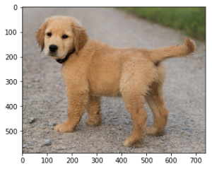

To demonstrate filtering effects, we’ll add random noise to the original image:

noised = (img + 0.2 * np.random.rand(*img.shape).astype(np.float32))
noised = noised.clip(0, 1)
plt.imshow(noised[:, :, [0, 1, 2]])
plt.title('Noisy Image')
plt.axis('off')
plt.show()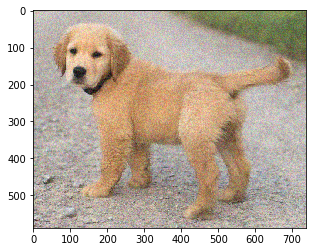

---

3. Gaussian Filtering — cv2.GaussianBlur

Theory

Gaussian filtering is the most commonly used linear smoothing filter. Its core idea is to convolve the image with a Gaussian kernel (a discretized 2D Gaussian function), where each pixel’s new value is a weighted average of its neighbors, with weights determined by a Gaussian distribution. Pixels closer to the center receive higher weights, while those farther away receive lower weights.

Gaussian filtering effectively removes Gaussian noise but blurs edges and fine details.

Syntax

cv2.GaussianBlur(src, ksize, sigmaX[, dst[, sigmaY[, borderType]]])

Parameters:

• src: Input image
• ksize: Gaussian kernel size, in the form (width, height), must be a positive odd number
• sigmaX: Gaussian standard deviation in the X direction
• sigmaY: Gaussian standard deviation in the Y direction; if set to 0, it is automatically computed from sigmaX

Code Example

gauss_blur = cv2.GaussianBlur(noised, (7, 7), 0)
plt.imshow(gauss_blur[:, :, [0, 1, 2]])
plt.title('Gaussian Blur Result')
plt.axis('off')
plt.show()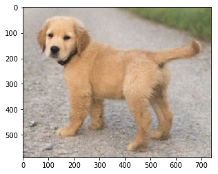

Use Cases

• Removing Gaussian noise
• Smoothing step in image preprocessing pipelines
• Reducing image noise before edge detection
• Scenarios where high image quality isn’t critical and fast smoothing is sufficient

---

4. Median Filtering — cv2.medianBlur

Theory

Median filtering is a non-linear filter. It replaces each pixel’s value with the median of all pixel values in its neighborhood. Median filtering is particularly effective against salt-and-pepper noise, because such noise manifests as extreme values (pure black or pure white), and the median operation naturally excludes outliers.

Unlike Gaussian filtering, median filtering preserves edge sharpness well while denoising.

Syntax

cv2.medianBlur(src, ksize[, dst])

Parameters:

• src: Input image (note: for certain data types, conversion to uint8 is required)
• ksize: Kernel size, must be a positive odd number (e.g., 3, 5, 7, 9…)

Code Example

median_blur = cv2.medianBlur((noised * 255).astype(np.uint8), 7)
plt.imshow(median_blur[:, :, [0, 1, 2]])
plt.title('Median Blur Result')
plt.axis('off')
plt.show()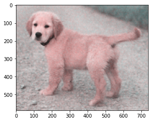

Use Cases

• Removing salt-and-pepper noise (best performance)
• Denoising scenarios that require sharp edge preservation
• Medical image processing
• Simple denoising preprocessing in embedded systems

---

5. Bilateral Filtering — cv2.bilateralFilter

Theory

Bilateral filtering is an edge-preserving non-linear filter. It considers two factors simultaneously:

1. Spatial distance (similar to Gaussian filtering) — closer pixels get higher weights
2. Color difference — more similar colors get higher weights

This means that while smoothing flat regions, bilateral filtering preserves edge information well and avoids mixing pixel values across edges.

Syntax

cv2.bilateralFilter(src, d, sigmaColor, sigmaSpace[, dst[, borderType]])

Parameters:

• src: Input image
• d: Diameter of each pixel neighborhood used during filtering. If negative, it is computed from sigmaSpace
• sigmaColor: Standard deviation in color space. Larger values mean more colors are considered similar
• sigmaSpace: Standard deviation in coordinate space. Larger values mean farther pixels are included as long as their colors are close enough

Code Example

bilat = cv2.bilateralFilter(noised, -1, 0.3, 10)
plt.imshow(bilat[:, :, [0, 1, 2]])
plt.title('Bilateral Filter Result')
plt.axis('off')
plt.show()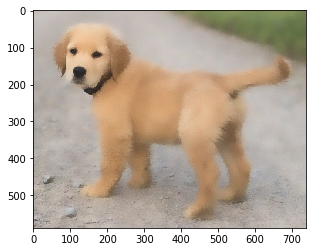

Use Cases and Trade-offs

• Denoising with edge preservation (e.g., portrait beauty filters)
• Removing texture while preserving structural information
• Trade-off: Slower computation than Gaussian and median filtering; not suitable for real-time processing of large images
• Parameter tuning is more complex and requires experimentation

---

6. Comparison of the Three Filters

Dimension	Gaussian	Median	Bilateral
Filter Type	Linear	Non-linear	Non-linear
Edge Preservation	Poor (blurs edges)	Good	Best
Gaussian Noise Removal	Good	Fair	Good
Salt-and-Pepper Noise Removal	Poor	Best	Fair
Computation Speed	Fast	Fast	Slow
Parameter Complexity	Low	Low	High
Recommended For	Fast smoothing, preprocessing	Salt-and-pepper noise removal	Edge-preserving denoising, beauty filters

How to choose?

• If you just need fast image smoothing → use Gaussian filtering
• If the image has salt-and-pepper noise → use median filtering
• If you need denoising while preserving sharp edges → use bilateral filtering

---

7. Sobel Edge Detection

Theory

The Sobel operator is a discrete differentiation operator used to compute an approximation of image intensity gradients. It combines Gaussian smoothing with differentiation, providing some noise suppression.

The Sobel operator computes gradients in the horizontal (x) and vertical (y) directions separately:

• dx: Detects vertical edges (horizontal gradient)
• dy: Detects horizontal edges (vertical gradient)

Code Example

import cv2
import numpy as np
import matplotlib.pyplot as plt

# Load image in grayscale
img = cv2.imread('dog.png', 0)

# Compute gradient approximations using the Sobel operator
dx = cv2.Sobel(img, cv2.CV_32F, 1, 0)
dy = cv2.Sobel(img, cv2.CV_32F, 0, 1)

# Display results
plt.figure(figsize=(10, 10))
plt.subplot(131)
plt.axis('off')
plt.title('Original Image')
plt.imshow(img, cmap='gray')
plt.subplot(132)
plt.axis('off')
plt.imshow(dx, cmap='gray')
plt.title(r'$\frac{dI}{dx}$')
plt.subplot(133)
plt.axis('off')
plt.title(r'$\frac{dI}{dy}$')
plt.imshow(dy, cmap='gray')
plt.tight_layout()
plt.show()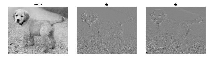

Syntax Reference

cv2.Sobel(src, ddepth, dx, dy[, dst[, ksize[, scale[, delta[, borderType]]]]])

• src: Input image
• ddepth: Output image depth (recommended: cv2.CV_32F or cv2.CV_64F)
• dx: Order of the derivative in x (1 means first-order derivative)
• dy: Order of the derivative in y
• ksize: Kernel size (1, 3, 5, 7), default is 3

Combining with Thresholding

You can combine Sobel results with thresholding to produce a binary edge map:

# Compute gradient magnitude
magnitude = np.sqrt(dx**2 + dy**2)
# Normalize
magnitude = magnitude / magnitude.max()
# Threshold
_, edges = cv2.threshold((magnitude * 255).astype(np.uint8), 50, 255, cv2.THRESH_BINARY)

---

8. Thresholding — cv2.threshold

Theory

Thresholding is the most basic image segmentation method. It compares each pixel against a threshold and assigns a new value based on the comparison result. OpenCV provides several threshold types, which can be grouped into two categories:

• Global thresholding: Uses the same threshold for all pixels
• Adaptive thresholding: Each pixel’s threshold depends on its surrounding pixel values

Global Threshold Types

ret, dst = cv2.threshold(src, thresh, maxval, type)

Type	Description
cv2.THRESH_BINARY	Pixel > thresh → maxval; otherwise → 0
cv2.THRESH_BINARY_INV	Pixel > thresh → 0; otherwise → maxval
cv2.THRESH_TRUNC	Pixel > thresh → thresh; otherwise unchanged
cv2.THRESH_TOZERO	Pixel > thresh → unchanged; otherwise → 0
cv2.THRESH_TOZERO_INV	Pixel > thresh → 0; otherwise unchanged
cv2.THRESH_OTSU	Automatically computes the optimal threshold using Otsu’s algorithm (combine with the above types)

Code Example

import cv2
import numpy as np
import matplotlib.pyplot as plt

img = cv2.imread('dog.png', 0)

# Apply simple binary threshold
thr, mask = cv2.threshold(img, 200, 1, cv2.THRESH_BINARY)
print('Threshold used:', thr)

# Apply adaptive threshold
adapt_mask = cv2.adaptiveThreshold(
    img, 255, cv2.ADAPTIVE_THRESH_MEAN_C, cv2.THRESH_BINARY_INV, 11, 10
)

# Display comparison
plt.figure(figsize=(10, 10))
plt.subplot(131)
plt.axis('off')
plt.title('Original Image')
plt.imshow(img, cmap='gray')
plt.subplot(132)
plt.axis('off')
plt.title('Binary Threshold')
plt.imshow(mask, cmap='gray')
plt.subplot(133)
plt.axis('off')
plt.title('Adaptive Threshold')
plt.imshow(adapt_mask, cmap='gray')
plt.tight_layout()
plt.show()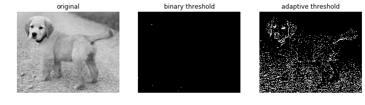

Adaptive Thresholding Explained

cv2.adaptiveThreshold computes an independent threshold for each pixel. With ADAPTIVE_THRESH_MEAN_C, for example, it calculates the mean of surrounding pixels and then subtracts a user-specified offset (10 in the example above) to determine that pixel’s threshold. This is particularly useful for images with uneven illumination.

---

9. Custom Filters

Theory

In addition to OpenCV’s built-in filtering functions, you can design your own filter kernels and apply them to images using cv2.filter2D. The key to custom filtering is constructing a 2D matrix (the kernel), where the values determine the weights assigned to each neighboring pixel during convolution.

Code Example: Sharpening Filter

import cv2
import numpy as np
import matplotlib.pyplot as plt

img = cv2.imread('dog.png')
img = cv2.cvtColor(img, cv2.COLOR_BGR2RGB)

KSIZE = 11
ALPHA = 2

# Create a Gaussian kernel using cv2.getGaussianKernel
kernel = cv2.getGaussianKernel(KSIZE, 0)
# Construct a sharpening kernel: negative Gaussian with an offset
kernel = -ALPHA * kernel @ kernel.T
kernel += 1 + ALPHA

# Apply the custom filter
filtered = cv2.filter2D(img, -1, kernel)

# Display comparison
plt.figure(figsize=(10, 10))
plt.subplot(121)
plt.axis('off')
plt.title('Original Image')
plt.imshow(img[:, :, [0, 1, 2]])
plt.subplot(122)
plt.axis('off')
plt.title('Sharpened')
plt.imshow(filtered[:, :, [0, 1, 2]])
plt.tight_layout(True)
plt.show()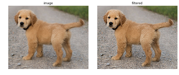

Other Commonly Used Custom Kernels

# Sharpening kernel (3x3)
sharpen_kernel = np.array([[ 0, -1,  0],
                           [-1,  5, -1],
                           [ 0, -1,  0]])

# Edge detection kernel (Laplacian)
laplacian_kernel = np.array([[0,  1, 0],
                             [1, -4, 1],
                             [0,  1, 0]])

# Emboss kernel
emboss_kernel = np.array([[-2, -1, 0],
                          [-1,  1, 1],
                          [ 0,  1, 2]])

# Apply
filtered = cv2.filter2D(img, -1, sharpen_kernel)

filter2D Syntax

cv2.filter2D(src, ddepth, kernel[, dst[, anchor[, delta[, borderType]]]])

• src: Input image
• ddepth: Output image depth (-1 means same as input)
• kernel: Convolution kernel (single-channel floating-point matrix)

---

10. Gabor Filters

Theory

A Gabor filter is a linear filter whose core is the product of a 2D Gaussian function and a cosine function (real-valued Gabor) or a complex exponential function (complex Gabor). Gabor filters can simultaneously capture frequency and orientation information, making them ideal for:

• Texture analysis: Detecting texture patterns in specific directions
• Edge detection: Detecting edges in known orientations
• Feature extraction: Widely used in face recognition and fingerprint recognition

Code Example

import cv2
import numpy as np
import matplotlib.pyplot as plt
import math

# Load image in grayscale and normalize
img = cv2.imread('dog.png', 0).astype(np.float32) / 255

# Create a real-valued Gabor kernel
kernel = cv2.getGaborKernel((21, 21), 5, 1, 10, 1, 0, cv2.CV_32F)
# Normalize the kernel
kernel /= math.sqrt((kernel * kernel).sum())

# Apply the filter
filtered = cv2.filter2D(img, -1, kernel)

# Display results
plt.figure(figsize=(10, 10))
plt.subplot(131)
plt.axis('off')
plt.title('Original Image')
plt.imshow(img, cmap='gray')
plt.subplot(132)
plt.title('Gabor Kernel')
plt.imshow(kernel, cmap='gray')
plt.subplot(133)
plt.axis('off')
plt.title('Filtered Result')
plt.imshow(filtered, cmap='gray')
plt.tight_layout()
plt.show()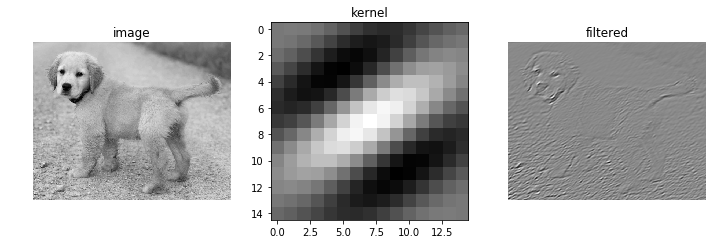

getGaborKernel Parameters

cv2.getGaborKernel(ksize, sigma, theta, lambd, gamma, psi[, ktype])

Parameter	Description
ksize	Kernel size, e.g., (21, 21)
sigma	Standard deviation of the Gaussian function
theta	Orientation of the Gabor function (in radians), 0 means vertical
lambd	Wavelength of the sinusoidal factor
gamma	Spatial aspect ratio (elongation of the ellipse)
psi	Phase offset
ktype	Kernel data type

By adjusting the theta parameter, you can detect edges in different directions. For example, setting theta = np.pi/4 detects edges at a 45° orientation.

---

11. Fourier Transform — cv2.dft

Theory

The Fourier Transform converts an image from the spatial domain to the frequency domain. In the frequency domain:

• Low-frequency components: Correspond to slowly varying regions (large flat areas)
• High-frequency components: Correspond to rapidly varying regions (edges, textures, noise)

By manipulating frequency components in the frequency domain, we can achieve powerful filtering effects:

• Low-pass filtering: Retain low frequencies, remove high frequencies → smoothing/blurring
• High-pass filtering: Retain high frequencies, remove low frequencies → sharpening/edge enhancement

Step 1: From Spatial Domain to Frequency Domain

import cv2
import numpy as np
import matplotlib.pyplot as plt

img = cv2.imread('dog.png', 0).astype(np.float32) / 255

# Apply Discrete Fourier Transform
fft = cv2.dft(img, flags=cv2.DFT_COMPLEX_OUTPUT)

# Shift low frequencies to the center
shifted = np.fft.fftshift(fft, axes=[0, 1])

# Compute magnitude spectrum and take log for visualization
magnitude = cv2.magnitude(shifted[:, :, 0], shifted[:, :, 1])
magnitude = np.log(magnitude)

plt.axis('off')
plt.imshow(magnitude, cmap='gray')
plt.title('Frequency Magnitude Spectrum')
plt.tight_layout()
plt.show()

Step 2: Verify the Inverse Transform

# Restore the image using the inverse transform
restored = cv2.idft(fft, flags=cv2.DFT_SCALE | cv2.DFT_REAL_OUTPUT)
plt.imshow(restored, cmap='gray')
plt.title('Image Restored via Inverse Transform')
plt.axis('off')
plt.show()

Step 3: Low-Pass Filtering in the Frequency Domain

# Re-run the DFT
fft = cv2.dft(img, flags=cv2.DFT_COMPLEX_OUTPUT)
fft_shift = np.fft.fftshift(fft, axes=[0, 1])

# Create a low-pass filter mask: keep only the central rectangular region (low-frequency components)
sz = 25
mask = np.zeros(fft_shift.shape, np.uint8)
mask[mask.shape[0]//2-sz:mask.shape[0]//2+sz,
     mask.shape[1]//2-sz:mask.shape[1]//2+sz, :] = 1
fft_shift *= mask

# Shift back
fft = np.fft.ifftshift(fft_shift, axes=[0, 1])

# Inverse DFT to convert back to spatial domain
filtered = cv2.idft(fft, flags=cv2.DFT_SCALE | cv2.DFT_REAL_OUTPUT)

# Display comparison
plt.figure(figsize=(10, 10))
plt.subplot(121)
plt.axis('off')
plt.title('Original Image')
plt.imshow(img, cmap='gray')
plt.subplot(122)
plt.axis('off')
plt.title('Image After Removing High Frequencies')
plt.imshow(filtered, cmap='gray')
plt.tight_layout()
plt.show()

High-Pass Filtering (Edge Preservation)

Simply invert the mask to achieve high-pass filtering:

# High-pass mask: remove central low frequencies, keep peripheral high frequencies
mask_hp = 1 - mask
fft_shift_hp = np.fft.fftshift(fft, axes=[0, 1])
fft_shift_hp *= mask_hp
fft_hp = np.fft.ifftshift(fft_shift_hp, axes=[0, 1])
filtered_hp = cv2.idft(fft_hp, flags=cv2.DFT_SCALE | cv2.DFT_REAL_OUTPUT)

---

12. Comprehensive Comparison Table

Method	Function	Domain	Type	Primary Use	Edge Preservation	Speed
Gaussian Blur	cv2.GaussianBlur	Spatial	Linear	Denoising, smoothing	Poor	Fast
Median Blur	cv2.medianBlur	Spatial	Non-linear	Salt-and-pepper noise removal	Good	Fast
Bilateral Filter	cv2.bilateralFilter	Spatial	Non-linear	Edge-preserving denoising	Best	Slow
Sobel Operator	cv2.Sobel	Spatial	Differential	Edge detection	—	Fast
Thresholding	cv2.threshold	Spatial	Segmentation	Image binarization	—	Fast
Custom Filter	cv2.filter2D	Spatial	Custom	Sharpening, embossing, etc.	Depends on kernel	Medium
Gabor Filter	cv2.getGaborKernel + filter2D	Spatial	Linear	Texture analysis, directional edges	Good	Medium
Fourier Transform	cv2.dft / cv2.idft	Frequency	Linear	Frequency-domain filtering	Depends on design	Medium

---

13. Summary and Best Practices

Key Takeaways

1. Analyze the noise type before choosing a filter: Use Gaussian filtering for Gaussian noise, median filtering for salt-and-pepper noise, and bilateral filtering when edge preservation is needed.

2. Parameter tuning is critical: The larger the kernel size (ksize), the stronger the smoothing effect — but also the more blur. Start with a small kernel (3×3) and increase gradually.

3. Combine preprocessing steps: A common pipeline is median/Gaussian denoising → Sobel/Canny edge detection → thresholding for a binary result.

4. Frequency-domain methods are ideal for global frequency operations: If you need precise control over specific frequency components (e.g., removing periodic noise), the Fourier Transform is the best choice.

5. Gabor filters excel at texture tasks: When detecting texture or edges in specific directions, Gabor filters provide dual selectivity in both orientation and frequency.

6. Custom filters offer maximum flexibility: With cv2.filter2D, you can implement any convolution-based filtering operation — from simple averaging to complex feature extraction.

Recommended Combinations

Task	Recommended Combination
General denoising	GaussianBlur → threshold
Salt-and-pepper noise removal	medianBlur → Canny
Edge detection	GaussianBlur → Sobel/Canny
Texture analysis	getGaborKernel + filter2D
Periodic noise removal	dft → frequency-domain mask → idft
Image sharpening	Custom sharpening kernel + filter2D
Beauty/skin smoothing	bilateralFilter

References

• OpenCV Image Filtering Module
• cv2.GaussianBlur
• cv2.medianBlur
• cv2.bilateralFilter
• cv2.Sobel
• cv2.threshold
• cv2.adaptiveThreshold
• cv2.getGaussianKernel
• cv2.filter2D
• cv2.getGaborKernel
• cv2.dft
• cv2.idft