The Complete Guide to OpenCV with Python: Reading, Displaying, Saving Images & Jupyter Setup

Introduction

OpenCV (Open Source Computer Vision Library) is the most widely used open-source computer vision library today. Originally developed by Intel, it is now maintained by the community. It provides interfaces for hundreds of image processing and vision algorithms — ranging from image I/O, geometric transformations, color space conversions, and feature detection to deep learning inference. OpenCV supports multiple languages including C++, Python, and Java. Among these, the Python bindings have become the go-to choice for getting started with computer vision, thanks to their clean syntax, seamless integration with NumPy arrays, and the interactive debugging experience offered by Jupyter Notebook.

This article is a complete beginner’s guide to OpenCV with Python, written for readers with zero prior experience. We’ll start from environment setup, then walk through image reading (cv.imread), window display (cv.imshow), Matplotlib display in Jupyter Notebook, image saving (cv.imwrite), inspecting image properties, troubleshooting common errors, and a full “read → process → save” hands-on pipeline. We’ll also include a bonus section on configuring Jupyter Lab to auto-start on a Jetson Nano — useful for those working on embedded vision projects.

After reading this article, you will be able to:

• Independently install and verify an OpenCV Python environment
• Read, display, and save images in various formats
• Correctly display images in Jupyter Notebook (including the color pitfall)
• Inspect and manipulate basic image properties
• Troubleshoot the 4 most common issues beginners encounter

Environment Setup

Installing the OpenCV Python package is straightforward — just use pip. It’s recommended to install NumPy and Matplotlib alongside it: NumPy is the underlying data structure for OpenCV’s Python interface (images are just NumPy arrays), and Matplotlib is used for visualizing images in Jupyter.

pip install opencv-python numpy matplotlib

If you also need OpenCV’s extended modules (which include patented algorithms like SIFT and SURF, plus some additional utility functions), install opencv-contrib-python instead:

pip install opencv-contrib-python numpy matplotlib

Note: Do not install opencv-python and opencv-contrib-python at the same time — they will conflict. Uninstall opencv-python first with pip uninstall opencv-python before installing the contrib version.

If you’re using Jupyter Notebook as your development environment, you’ll also need to install Jupyter:

pip install jupyterlab

Once installed, run jupyter lab to launch the browser-based interactive interface.

Version Check

After importing OpenCV, the first thing to do is check the version number:

import cv2
print(cv2.__version__)

Example output:

4.10.0

A common question: Why is the Python import name cv2 instead of opencv or cv?

This is simply a historical artifact. cv2 originally stood for “the OpenCV Python 2 interface,” but even though OpenCV has long moved to version 4.x and Python 2 has been officially deprecated, the module name has stuck. So remember: cv2 does not mean “OpenCV version 2” — it’s just the module name. The actual version must be checked via cv2.__version__.

cv.imread — Reading Images

cv2.imread() is the core function in OpenCV for reading images from files. Its signature is:

img = cv2.imread(filename[, flags])

• filename: Path to the image file; supports both relative and absolute paths
• flags: Optional parameter specifying the read mode

Read Modes (flags)

Flag Constant	Meaning
cv2.IMREAD_COLOR (default)	Always reads as 3-channel BGR color
cv2.IMREAD_GRAYSCALE	Always reads as single-channel grayscale
cv2.IMREAD_UNCHANGED	Preserves all original channels, including PNG alpha transparency
cv2.IMREAD_ANYDEPTH	Preserves image bit depth (e.g., 16-bit, 32-bit)

Basic Examples

import cv2

# Default color read
img = cv2.imread('example.jpeg')

# Grayscale read
img_gray = cv2.imread('example.jpeg', cv2.IMREAD_GRAYSCALE)

# Read with alpha channel preserved
img_rgba = cv2.imread('example.png', cv2.IMREAD_UNCHANGED)

Return Value Type

cv2.imread() returns a NumPy ndarray (multi-dimensional array). You can quickly inspect it with the following attributes:

import cv2
img = cv2.imread('example.jpeg')

print('shape:', img.shape)   # (height, width, channels), e.g. (147, 342, 3)
print('dtype:', img.dtype)   # uint8 (each pixel 0–255)
print('type:', type(img))    # <class 'numpy.ndarray'>

A few key points:

• The shape order is (height, width, channels), not (width, height) — this is the opposite of PIL/Pillow and a common source of confusion for beginners
• The default dtype is uint8, meaning each pixel value ranges from 0 to 255. Some special images (e.g., HDR, medical imaging) may be float32 (0–1) or uint16
• The channel order is BGR, not the more common RGB! This is a legacy design choice in OpenCV. When displaying with Matplotlib, you must convert manually

Error Handling: What If the File Doesn’t Exist?

Here’s a critical gotcha: cv2.imread() does not raise an error or throw an exception when the file doesn’t exist or the path is wrong — it silently returns None. If you then try to access None.shape, Python will throw an AttributeError, leaving beginners puzzled.

img = cv2.imread('typo_in_filename.jpeg')
print(img)  # None
# Now print(img.shape) will error: AttributeError: 'NoneType' object has no attribute 'shape'

Recommended defensive pattern:

img = cv2.imread('example.jpeg')
if img is None:
    raise FileNotFoundError(f"Unable to read image, please check the path: example.jpeg")
print('shape:', img.shape)

cv.imshow — Window Display

cv2.imshow() displays an image in a standalone window, suitable for use in local Python scripts (not Jupyter).

cv2.imshow(winname, mat)

• winname: Window name string
• mat: Image data (NumPy array)

Complete Example

import cv2

img = cv2.imread("cook.jpeg")
if img is None:
    print("Image failed to load")
    exit(1)

# Display the image
cv2.imshow("Original image", img)

# Wait for a key press, in milliseconds. 2000 means wait 2 seconds
# 0 means wait indefinitely until a key is pressed
cv2.waitKey(2000)

# Destroy all windows created by OpenCV
cv2.destroyAllWindows()

Key Functions Reference

Function	Purpose
cv2.imshow(winname, img)	Creates/refreshes a window named winname and displays the image
cv2.waitKey(delay)	Waits for a key event. Returns -1 if no key is pressed within delay ms; returns the ASCII value of the key if pressed. This function is the core of OpenCV’s GUI event loop — without it, the window won’t refresh
cv2.destroyAllWindows()	Destroys all windows created by OpenCV
cv2.destroyWindow(winname)	Destroys a single window with the specified name
cv2.namedWindow(winname, flags)	Pre-creates a window; use cv2.WINDOW_NORMAL to make it freely resizable

Creating a Resizable Window

By default, windows created by cv2.imshow() are fixed to the image dimensions — large images will be clipped. To make the window resizable, create it first with cv2.namedWindow():

cv2.namedWindow("Large image", cv2.WINDOW_NORMAL)
cv2.imshow("Large image", img)
cv2.waitKey(0)
cv2.destroyAllWindows()

The Jupyter Notebook Pitfall

When using cv2.imshow() + cv2.waitKey() in Jupyter Notebook, the popup window cannot be closed normally — the only fix is to force-restart the kernel. This is because OpenCV’s GUI event loop conflicts with Jupyter’s asyncio event loop.

Solution: Don’t use cv2.imshow() in Jupyter. Instead, use the Matplotlib approach described below.

Matplotlib Display in Jupyter

Matplotlib is Python’s most popular plotting library and the official visualization tool for NumPy. In Jupyter Notebook, we use matplotlib.pyplot (commonly abbreviated as plt) to display images.

import cv2
import matplotlib.pyplot as plt

img = cv2.imread("cook.jpeg")
plt.imshow(img)
plt.axis("off")   # Hide axes
plt.show()

A single line plt.imshow(img) displays the image inline in the notebook cell output — no window lifecycle management needed, making it very developer-friendly for debugging.

Pitfall 1: Incorrect BGR Color Display

After running the code above, many beginners immediately notice a problem: the colors look wrong! Reds appear blue, blues appear red.

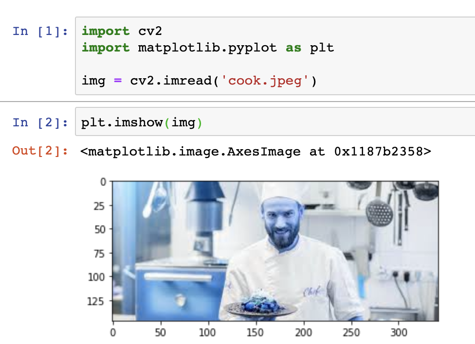
The reason is that OpenCV reads images in BGR channel order, while Matplotlib expects RGB by default. The two libraries have opposite channel conventions.

Solution: Manually convert BGR to RGB after reading

import cv2
import matplotlib.pyplot as plt

img_bgr = cv2.imread("cook.jpeg")
img_rgb = cv2.cvtColor(img_bgr, cv2.COLOR_BGR2RGB)  # BGR → RGB
plt.imshow(img_rgb)
plt.axis("off")
plt.show()

After conversion, the colors display correctly. Remember: whenever an image read by OpenCV is to be displayed by Matplotlib, you must perform a cv2.COLOR_BGR2RGB conversion.

Pitfall 2: Grayscale Images Displayed as False Color

A grayscale image read with cv2.IMREAD_GRAYSCALE, when passed directly to plt.imshow(), will appear as a purple-green “heatmap” (Matplotlib applies the viridis false-color colormap by default).

img_gray = cv2.imread("example.jpeg", cv2.IMREAD_GRAYSCALE)
plt.imshow(img_gray)   # Wrong: displayed as false color

Solution: Explicitly specify cmap="gray"

img_gray = cv2.imread("example.jpeg", cv2.IMREAD_GRAYSCALE)
plt.imshow(img_gray, cmap="gray")   # Correct: displayed as grayscale
plt.axis("off")
plt.show()

Multi-Image Comparison: Using subplots

When doing image processing, you often need to compare the original with the processed result. plt.subplots() creates a multi-subplot canvas in a single line:

import cv2
import matplotlib.pyplot as plt

img_bgr = cv2.imread("cook.jpeg")
img_rgb = cv2.cvtColor(img_bgr, cv2.COLOR_BGR2RGB)
img_gray = cv2.cvtColor(img_rgb, cv2.COLOR_RGB2GRAY)

fig, axes = plt.subplots(1, 3, figsize=(12, 4))
axes[0].imshow(img_rgb);    axes[0].set_title("Original (RGB)");  axes[0].axis("off")
axes[1].imshow(img_gray, cmap="gray"); axes[1].set_title("Grayscale"); axes[1].axis("off")
axes[2].hist(img_gray.ravel(), 256, [0, 256]); axes[2].set_title("Histogram")
plt.tight_layout()
plt.show()

cv.imwrite — Saving Images

cv2.imwrite() saves an image to a file:

retval = cv2.imwrite(filename, img[, params])

• filename: Save path (file extension determines the format)
• img: Image to save (NumPy array)
• params: Optional encoding parameters

Supported Formats

The save formats supported by OpenCV depend on the image codecs installed on your system. Common formats include: .jpg / .jpeg, .png, .bmp, .tif / .tiff, .webp. The file extension automatically determines the encoding format.

Lossless Saving: PNG

PNG uses lossless compression, preserving all image data. The third parameter controls the compression level:

import cv2
img = cv2.imread("dashen.jpeg")

# Save as PNG, lossless
cv2.imwrite('dashen.png', img)

# Save as PNG with a specific compression level (0=no compression, 9=max compression)
# Note: compression only affects file size, not image quality (PNG is always lossless)
cv2.imwrite('dashen_compressed.png', img, [cv2.IMWRITE_PNG_COMPRESSION, 0])

# Verify losslessness: re-read and compare with the original
img_png = cv2.imread("dashen_compressed.png")
assert img_png.shape == img.shape
assert (img_png == img).all(), "PNG should be lossless; data should be identical"
print("PNG lossless save verification passed ✓")

Lossy Compression: JPEG

JPEG uses lossy compression, which can significantly reduce file size at the cost of some image detail. The third parameter controls quality:

# Save JPEG at default quality
cv2.imwrite('dashen.jpg', img)

# Specify JPEG quality (0–100; higher = better quality, larger file)
cv2.imwrite('dashen_high_quality.jpg', img, [cv2.IMWRITE_JPEG_QUALITY, 95])
cv2.imwrite('dashen_low_quality.jpg', img, [cv2.IMWRITE_JPEG_QUALITY, 30])

Quality parameter guidelines (rule of thumb):

JPEG_QUALITY	Use Case
95–100	High-quality archival, printing
85–95	Web display, everyday use
60–85	Thumbnails, mobile loading
30–60	Preview images, quality not a priority

Note: Channel Order

cv2.imwrite() expects input in BGR channel order (matching cv2.imread()). If you previously converted to RGB with cv2.COLOR_BGR2RGB for Matplotlib display, remember to save using the BGR version, or convert back to BGR first:

img_bgr = cv2.imread("cook.jpeg")
img_rgb = cv2.cvtColor(img_bgr, cv2.COLOR_BGR2RGB)  # For Matplotlib display
# ... do some processing ...
cv2.imwrite("processed.jpg", img_bgr)  # Save with the BGR version — correct

Image Properties in Detail

An image loaded by OpenCV is simply a NumPy multi-dimensional array, so all NumPy attributes apply.

Basic Attributes

import cv2
img = cv2.imread("example.jpeg")

print("shape:", img.shape)   # (height, width, channels), e.g. (480, 640, 3)
print("dtype:", img.dtype)   # uint8
print("size:", img.size)     # Total pixel count = height × width × channels, e.g. 921600
print("type:", type(img))    # <class 'numpy.ndarray'>
print("ndim:", img.ndim)     # Number of dimensions: color=3, grayscale=2

Key concepts:

• shape[0] = Image height (number of rows)
• shape[1] = Image width (number of columns)
• shape[2] = Number of channels (this dimension doesn’t exist for grayscale images)

Accessing Individual Pixels

The image array can be indexed directly to access pixel values:

# Access the pixel at (row=100, col=200) — note: row first, then column
pixel = img[100, 200]
print("BGR values:", pixel)    # e.g. [123 45 67]
print("Blue:",  pixel[0])
print("Green:", pixel[1])
print("Red:",   pixel[2])

# Modify a single pixel
img[100, 200] = [255, 0, 0]    # Set this pixel to pure blue

Performance tip: Pixel-by-pixel access is extremely slow in Python. In real projects, prefer NumPy’s vectorized operations (e.g., img[img > 128] = 255) or OpenCV’s built-in functions.

Region of Interest (ROI)

NumPy’s slicing syntax lets you crop any rectangular region of an image directly:

img = cv2.imread("example.jpeg")

# Crop ROI: rows 50–200, columns 100–300
roi = img[50:200, 100:300]

print("roi shape:", roi.shape)   # (150, 200, 3)

# You can process the ROI independently
roi_gray = cv2.cvtColor(roi, cv2.COLOR_BGR2GRAY)

# You can also write the processed ROI back into the original image
img[50:200, 100:300] = roi_gray[..., None]   # Note: dimension alignment

Jupyter Auto-Start Configuration (Jetson Nano / Raspberry Pi, etc.)

When working on embedded vision projects, you often want your dev board (e.g., Jetson Nano, Raspberry Pi) to automatically launch Jupyter Lab on boot — saving you the trouble of SSH-ing in and starting it manually each time. Below is a method using a systemd service to achieve auto-start.

This method works on any Linux system using systemd, including Jetson Nano, Raspberry Pi, Ubuntu Server, Atomic PI, and more.

Step 1: Find the Jupyter Install Path

which jupyter-lab
# Example output: /home/bbot/.local/bin/jupyter-lab

Note this path — you’ll need it in the service file.

Step 2: Create the systemd Service File

sudo nano /etc/systemd/system/jupyter.service

Fill in the following content (be sure to change User, ExecStart, and WorkingDirectory to match your actual paths):

[Unit]
Description=Jupyter Lab
After=network.target

[Service]
Type=simple
User=bbot
ExecStart=/home/bbot/.local/bin/jupyter-lab --port 8888 --no-browser --ip=0.0.0.0
WorkingDirectory=/home/bbot/Notebook
Restart=on-failure
RestartSec=5

[Install]
WantedBy=multi-user.target

A few notes:

• --no-browser: Don’t open a browser on the server
• --ip=0.0.0.0: Allow access from other devices on the LAN (default only allows localhost)
• Restart=on-failure: Auto-restart on crash

Step 3: Enable and Start the Service

sudo systemctl daemon-reload
sudo systemctl enable jupyter    # Start on boot
sudo systemctl start jupyter     # Start immediately

Step 4: Check Service Status

sudo systemctl status jupyter

Seeing active (running) means the service is running properly. After rebooting the dev board, Jupyter Lab will automatically start on port 8888, and computers on the LAN can access it at http://<board-IP>:8888.

Frequently Asked Questions

Q1: cv2 is not cv2 or No module named 'cv2'

This is usually caused by one of the following:

• OpenCV not installed: pip install opencv-python
• Multiple Python environments conflicting: pip installed to environment A, but you’re running Python from environment B. Use which python and which pip to confirm the paths match, or use python -m pip install opencv-python instead
• Both opencv-python and opencv-contrib-python installed simultaneously: Uninstall one, keeping only one

Q2: Image loads as None / accessing shape throws an error

When the file path is wrong, cv2.imread() does not throw an exception — it returns None. Always add a check:

img = cv2.imread(path)
if img is None:
    print(f"Failed to load: {path}")

Common path issues:

• Using a relative path but the current working directory is wrong (check with os.getcwd())
• Path contains non-ASCII characters (some OpenCV versions don’t support this; use cv2.imdecode() instead)
• Backslash issues on Windows: use forward slashes / or raw strings r"C:\path\to\img.jpg"

Q3: Matplotlib displays the wrong colors

As mentioned above, OpenCV reads images in BGR, while Matplotlib expects RGB. Convert with cv2.cvtColor(img, cv2.COLOR_BGR2RGB).

Q4: Grayscale image displays as purple-green

Passing a grayscale image directly to plt.imshow() triggers the default false-color colormap. Add cmap="gray" to fix it:

plt.imshow(gray_img, cmap="gray")

Q5: OpenCV version conflicts / function not found

• Some functions are exclusive to opencv-contrib-python (e.g., cv2.SIFT_create()). If you installed the regular opencv-python, you’ll get an AttributeError
• Upgrade OpenCV: pip install -U opencv-python
• Check current version: print(cv2.__version__)

Complete Hands-On Example

Below is a full “read → process → save” pipeline that ties together everything covered in this article:

import cv2
import matplotlib.pyplot as plt

# ===== 1. Read the image =====
img_path = "example.jpeg"
img_bgr = cv2.imread(img_path)
if img_bgr is None:
    raise FileNotFoundError(f"Unable to read image: {img_path}")
print(f"Original shape: {img_bgr.shape}, dtype: {img_bgr.dtype}")

# ===== 2. Convert to RGB for display =====
img_rgb = cv2.cvtColor(img_bgr, cv2.COLOR_BGR2RGB)

# ===== 3. Image processing =====
# Convert to grayscale
img_gray = cv2.cvtColor(img_bgr, cv2.COLOR_BGR2GRAY)

# Gaussian blur for noise reduction
img_blur = cv2.GaussianBlur(img_gray, (5, 5), 0)

# Canny edge detection
edges = cv2.Canny(img_blur, threshold1=50, threshold2=150)

# Crop ROI (top-left 200×200 region of the original)
roi = img_rgb[0:200, 0:200]

# ===== 4. Multi-image comparison display =====
fig, axes = plt.subplots(2, 3, figsize=(14, 8))
titles = ["Original", "Grayscale", "Blurred", "Edges", "ROI", "Histogram"]

axes[0, 0].imshow(img_rgb);     axes[0, 0].set_title(titles[0]); axes[0, 0].axis("off")
axes[0, 1].imshow(img_gray, cmap="gray"); axes[0, 1].set_title(titles[1]); axes[0, 1].axis("off")
axes[0, 2].imshow(img_blur, cmap="gray"); axes[0, 2].set_title(titles[2]); axes[0, 2].axis("off")
axes[1, 0].imshow(edges, cmap="gray");    axes[1, 0].set_title(titles[3]); axes[1, 0].axis("off")
axes[1, 1].imshow(roi);         axes[1, 1].set_title(titles[4]); axes[1, 1].axis("off")
axes[1, 2].hist(img_gray.ravel(), 256, [0, 256]); axes[1, 2].set_title(titles[5])

plt.tight_layout()
plt.show()

# ===== 5. Save results =====
cv2.imwrite("output_gray.jpg", img_gray, [cv2.IMWRITE_JPEG_QUALITY, 95])
cv2.imwrite("output_edges.png", edges)   # PNG lossless
print("Processing results saved")

# ===== 6. Verify the save =====
img_saved = cv2.imread("output_gray.jpg")
print(f"Saved shape: {img_saved.shape}")

This code demonstrates:

• Defensive reading (checking for None)
• BGR↔RGB color conversion
• Multiple image processing operations (grayscale, blur, edge detection, ROI cropping)
• Matplotlib multi-image comparison display (including grayscale cmap handling)
• Saving results in different formats and quality levels
• Post-save verification

Summary

This article started from environment setup and version checking, then systematically covered the four core operations for getting started with OpenCV in Python: cv2.imread for reading images, cv.imshow for window display, Matplotlib for Jupyter display, and cv2.imwrite for saving images. We also dug into the most common pitfalls for beginners: BGR vs. RGB color order, cmap="gray" for grayscale images, and cv2.imread returning None silently on failure.

Let’s recap the key takeaways:

1. The import is called cv2, but it doesn’t mean version 2 — use cv2.__version__ to check the actual version
2. cv2.imread() returns None on failure — always check, or AttributeError will find you
3. OpenCV reads images in BGR — you must convert with cv2.cvtColor(img, cv2.COLOR_BGR2RGB) before passing to Matplotlib
4. Grayscale images need cmap="gray" — otherwise Matplotlib will display them as purple-green false color
5. cv2.imwrite() picks the format by extension — PNG is lossless, JPEG lets you specify quality
6. Don’t use cv2.imshow() in Jupyter — use Matplotlib instead to avoid GUI event loop conflicts

Once you’ve mastered these fundamentals, you’ll have the foundation needed for any complex image processing task with OpenCV. Next steps include geometric transformations, color spaces, morphological operations, and contour detection — topics we’ll cover in subsequent articles.

The full source code is available for practice alongside this article. If you have questions or find errors, feel free to leave a comment. Happy OpenCV learning!